Programmatic Inference for State-Space Models

A tour of structure-agnostic and structure-aware tooling

Adrien Corenflos

Why this talk

State-space models, everywhere:

• Tracking, navigation
• Econometrics, finance
• Epidemiology
• Robotics, control
• Generative AI (diffusion models, RNNs, LLMs, …)

Inference software: scattered across ecosystems, philosophies, levels of abstraction.

Goal: a map of what exists, and our efforts to form a real probabilistic programming ecosystem for SSMs in Python.

Roadmap

1. A quick landscape tour: why the ecosystem looks the way it does
2. Deep dive: cuthbert and dynestyx
3. cuthbert in the wild: predicting the World Cup

What is a state-space model?

A latent Markov process \(x_t\), observed indirectly through \(y_t\):

\[ x_t \mid x_{t-1} \sim p(x_t \mid x_{t-1}) \qquad y_t \mid x_t \sim p(y_t \mid x_t) \]

Three inference targets, recurring throughout:

• Filtering: \(p(x_t \mid y_{1:t})\)
• Smoothing: \(p(x_{1:T} \mid y_{1:T})\) or \(p(x_t \mid y_{1:T})\)
• Parameter estimation: \(p(\theta \mid y_{1:T})\)

The landscape: R, Julia, Python

Ecosystem	Character
R	Mature, classical/Bayesian SSM tooling: KFAS, dlm, bsts
Julia	General PPLs (Turing.jl), growing SSM-specific support
Python	Richest ecosystem, most fragmented: general PPLs and SSM-specific libraries side by side

Rest of the talk: Python.

Structure-agnostic vs. structure-aware

• Structure-agnostic: engine sees an opaque log-density. Markov structure, if any, invisible to it. (Stan, generic MCMC)
• Structure-aware, general graph: dependency graph explicit. Engine unaware it’s a state-space model specifically. (PyMC, NumPyro, Pyro, TensorFlow Probability)
• Structure-aware, SSM-specific: engine built around the SSM factorization, exploits it directly. (cuthbert, dynestyx, dynamax)

Structure-agnostic vs. structure-aware, in code

Agnostic (Stan): the recursion, written by hand.

model {
  for (t in 2:n)
    mu[t] ~ normal(mu[t-1], sigma_level);
  y ~ normal(mu, sigma_irreg);
}

Aware, general-graph (TensorFlow Probability): the SSM is a first-class Distribution without any hand-rolled recursion.

model = tfd.HiddenMarkovModel(
    initial_distribution=initial_distribution,
    transition_distribution=transition_distribution,
    observation_distribution=observation_distribution,
    num_steps=7)

model.mean(); model.log_prob(tf.zeros(shape=[7]))

Same split shows up elsewhere: R’s KFAS is declarative like TFP here; PyMC’s pytensor.scan is hand-rolled like Stan, though its newer pymc-extras.statespace layer grows an SSM-native shortcut on top, but more focused on the model definition (classical time series superposition).

Why structure matters

Time-decomposition often allows for algorithms that run in \(O(T)\) rather than \(O(T^3)\), or \(O(\log T)\) rather than \(O(T)\), both in memory and in compute (depending on the hardware). The SSM factorization is a strong inductive bias: it allows for inference methods that are computationally optimal.

Karjalainen, Lee, Singh & Vihola, “On the Forgetting of Particle Filters” (arXiv:2309.08517): the SSM / Feynman–Kac mixing structure gives particle filters a provably optimal \(O(\log N)\) forgetting of initialisation. Generic MCMC/VI on an unstructured joint posterior has no analogue of this guarantee.

And it’s not just theory: Rao–Blackwellization, finite/discrete truncations, sigma-points methods, and particle methods all pre-date today’s SSM-agnostic software, born out of application-driven approximation rather than a “one algorithm fits any density” philosophy.

dynamax

JAX library, structure-aware, SSM-specific. Model classes, with inference methods attached to each:

import jax.random as jr
from dynamax.hidden_markov_model import GaussianHMM

key1, key2, key3 = jr.split(jr.PRNGKey(0), 3)
num_states, emission_dim, num_timesteps = 3, 2, 1000

hmm = GaussianHMM(num_states, emission_dim)
true_params, _ = hmm.initialize(key1)
true_states, emissions = hmm.sample(true_params, key2, num_timesteps)

params, props = hmm.initialize(key3, method="kmeans", emissions=emissions)
params, lls = hmm.fit_em(params, props, emissions, num_iters=20)

post = hmm.smoother(params, emissions)

Model classes: Gaussian and non-Gaussian HMMs, linear and nonlinear Gaussian SSMs. Inference and learning: methods on the model instance (.sample, .fit_em, .smoother).

Model and inference, coupled

dynamax’s OO layer ties each model class to its own inference methods: GaussianHMM(...).smoother(...), LinearGaussianSSM(...).filter(...). Swapping inference algorithm means switching model class, or extending the hierarchy.

dynestyx’s docs discuss the coupling of tools:

One drawback of this suite of methods [dynamax, cd-dynamax, PFJax] is a varied set of APIs, with model code that is tightly coupled with the resulting inference method. In dynestyx, we offer a large variety of different inference methods under the same roof in a unified, abstract API.

Separating model from inference: BlackJAX

BlackJAX: deliberately structure-agnostic by design. Only ever sees a plain log-density function:

adapt = blackjax.window_adaptation(
    blackjax.nuts, logdensity_fn, target_acceptance_rate=0.8
)
(last_state, parameters), _ = adapt.run(
    warmup_key, initial_position, num_warmup)
kernel = blackjax.nuts(logdensity_fn, **parameters).step

BlackJAX on composability: “Sampling algorithms are too often integrated into PPLs and not decoupled from the rest of the framework […]. Their implementation is most of the time monolithic and it is impossible to reuse parts of the algorithm to build custom kernels.”

cuthbert’ stems from the same philosophy: decoupling model and inference. But unlike BlackJAX, cuthbert is structure-aware: it knows it’s dealing with a state-space model, and exploits that structure to run inference efficiently.

Enter cuthbert

A JAX library for SSM inference: filtering, smoothing, static parameter estimation.

Explicitly not a PPL: a stated non-goal.

cuthbert is not a probabilistic programming language (PPL). But can easily compose with dynamax, distrax, numpyro and pymc in a similar way to how blackjax does.

Functional API:

The only classes in cuthbert are NamedTuples and Protocols. All functions are pure, and work seamlessly with jax.grad, jax.jit, jax.vmap.

BlackJAX: inference-only and structure-agnostic. cuthbert: inference-only and SSM-structure-aware.

cuthbert: building a filter

from jax import numpy as jnp
from cuthbert.gaussian import kalman

def build_car_tracking_filter(m0, chol_P0, F, c, chol_Q, H, d, chol_R, ys):
    def get_init_params(model_inputs):
        return m0, chol_P0

    def get_dynamics_params(model_inputs):
        return F, c, chol_Q

    def get_observation_params(model_inputs):
        return H, d, chol_R, ys[model_inputs - 1]

    filter_obj = kalman.build_filter(
        get_init_params, get_dynamics_params, get_observation_params
    )
    model_inputs = jnp.arange(len(ys) + 1)
    return filter_obj, model_inputs

The pattern: get_dynamics_params / get_observation_params, pure functions of a model_inputs pytree. Same functions, reusable across Kalman, EKF/UKF, or particle-filter backends.

Decouples model and inference method.

cuthbert: running the filter

from cuthbert import filter

filter_obj, model_inputs = build_car_tracking_filter(
    m0, chol_P0, F, c, chol_Q, H, d, chol_R, ys)

init_state = filter_obj.init_prepare(model_inputs[0])
filtered_states = filter(filter_obj, model_inputs[1:], init_state,
                          parallel=True)
means = filtered_states.mean

parallel=True: \(O(\log T)\) temporal-parallel filtering.

cuthbert: what’s under the hood

One unified interface (init_prepare / filter_prepare / filter_combine) behind every backend:

Model class	Backend
Linear-Gaussian	Kalman/RTS (√-form, parallel-in-time)
Nonlinear-Gaussian	EKF / UKF / CKF / GHKF
Discrete / finite-state	Forward-backward, Baum–Welch
General nonlinear	Particle filter (SMC) + FFBSi smoothing
High-dimensional	Ensemble Kalman Filter + localization
Factorized dynamics	Factorial SSMs (Duffield et al. 2024)

Swapping inference method: swapping the build_filter(...) call. Everything downstream (cuthbert.filter, cuthbert.smoother): unchanged.

cuthbert: predict/update in \(O(\log T)\)

Classical recursion: two named steps, called sequentially. The parallel-in-time reformulation (Särkkä & García-Fernández, 2021) repackages both into one associative element:

class FilterScanElement(NamedTuple):
    A: Array; b: Array; U: Array
    eta: Array; Z: Array; ell: ScalarArray

def filtering_operator(elem_i, elem_j) -> FilterScanElement:
    ...   # QR-type triangularizations, forward/backward info combined
    return FilterScanElement(A, b, U, eta, Z, ell)

Filter only exposes filter_prepare (element construction) plus filter_combine (this operator). Feed filter_combine to jax.lax.associative_scan (or just a standard scan): compute drops from \(O(T)\) to \(O(\log T)\) given enough parallel workers.

Scope currently: Discrete/Gaussian filters/smoothers only; particle filters/ensemble Kalman stay sequential (for now).

dynestyx: cuthbert’s model-authoring layer

An extension of NumPyro, same decoupling philosophy one level up: dynestyx uses cuthbert as one of its three inference backends (alongside BlackJAX and cd-dynamax). dsx.sample(...) dispatches differently depending on the active handler: Simulator() / Filter() / LatentPathBuilder().

def continuous_time_lti_gaussian_model(rho=None, obs_times=None, obs_values=None):
    rho = numpyro.sample("rho", dist.Uniform(0.0, 5.0), obs=rho)
    A = jnp.array([[-1.0, 0.0], [rho, -1.0]])

    dynamics = DynamicalModel(
        initial_condition=dist.MultivariateNormal(
            loc=jnp.zeros(2), covariance_matrix=1.0**2 * jnp.eye(2)),
        state_evolution=ContinuousTimeStateEvolution(
            drift=lambda x, u, t: A @ x,
            diffusion=ScalarDiffusion(1.0, bm_dim=2)),
        observation_model=LinearGaussianObservation(
            H=jnp.array([[0.0, 1.0]]), R=jnp.array([[0.15**2]])),
    )
    return dsx.sample("f", dynamics, obs_times=obs_times, obs_values=obs_values)

dsx.sample ties together ordinary MCMC sampling for parameters (rho) and a DynamicalModel plus chosen backend for the dynamics.

Picking cuthbert as the inference engine, from dynestyx

Backend choice: explicit, per algorithm, via a filter_source field on the config dataclass, not automatic structural dispatch. EnKF and particle filtering: cuthbert-only. Kalman/EKF: either backend, and parallel-in-time Kalman filter specifically requires filter_source="cuthbert".

with Filter(filter_config=KFConfig(filter_source="cuthbert")):
    filtered = dsx.condition("lgssm", lgssm,
                              obs_times=obs_times, obs_values=y)

filtered_means = filtered.states.mean
print(filtered.marginal_loglik)

Under the hood: an adapter translates the DynamicalModel into the get_init_params / get_dynamics_params / get_observation_params closures of cuthbert’s kalman.build_filter.

Design choices, side by side

	cuthbert	dynestyx
Role	Inference engine	Model authoring + inference selection
Built on	Plain JAX	NumPyro + effectful
API style	Pure functions only	Effect handlers over DynamicalModel
Model classes	Gaussian → discrete → particle → ensemble → factorial	Discrete- & continuous-time, (non)linear, (non)Gaussian
Inference selection	Pick a backend module	Config objects (filter_source, …)
Relationship	One of dynestyx’s backends	Depends on cuthbert directly

cuthberto-carlos: the live site

state-space-models.github.io/cuthberto-carlos.

cuthberto-carlos: predicting the World Cup

cuthbert’s factorial support, in the wild: predicting the 2026 FIFA World Cup, live, at state-space-models.github.io/cuthberto-carlos.

Follows Duffield, Power & Rimella, “A state-space perspective on modelling and inference for online skill rating” (JRSS-C, 2024). One attack/defence pair per team, evolving over time (Ornstein-Uhlenbeck dynamics), joined per fixture into a single factorial state-space model with a bivariate Poisson observation:

\[ p(x^i_k \mid x^i_{k-1}) = N\left(x^i_k \mid \mu_0 + \phi_k(x^i_{k-1}-\mu_0),\ Q_k\right) \]

\[ p(y_k \mid x^i_k, x^j_k) = \mathrm{BivPoisson}(y_k \mid x^i_k, x^j_k, \alpha, \beta) \]

Built with the same get_*_params pattern from earlier, wrapped in cuthbert.factorial: one 2-D state per team, joined per match, filtered with the moments (EKF-style) backend.

cuthberto-carlos: results vs. Polymarket

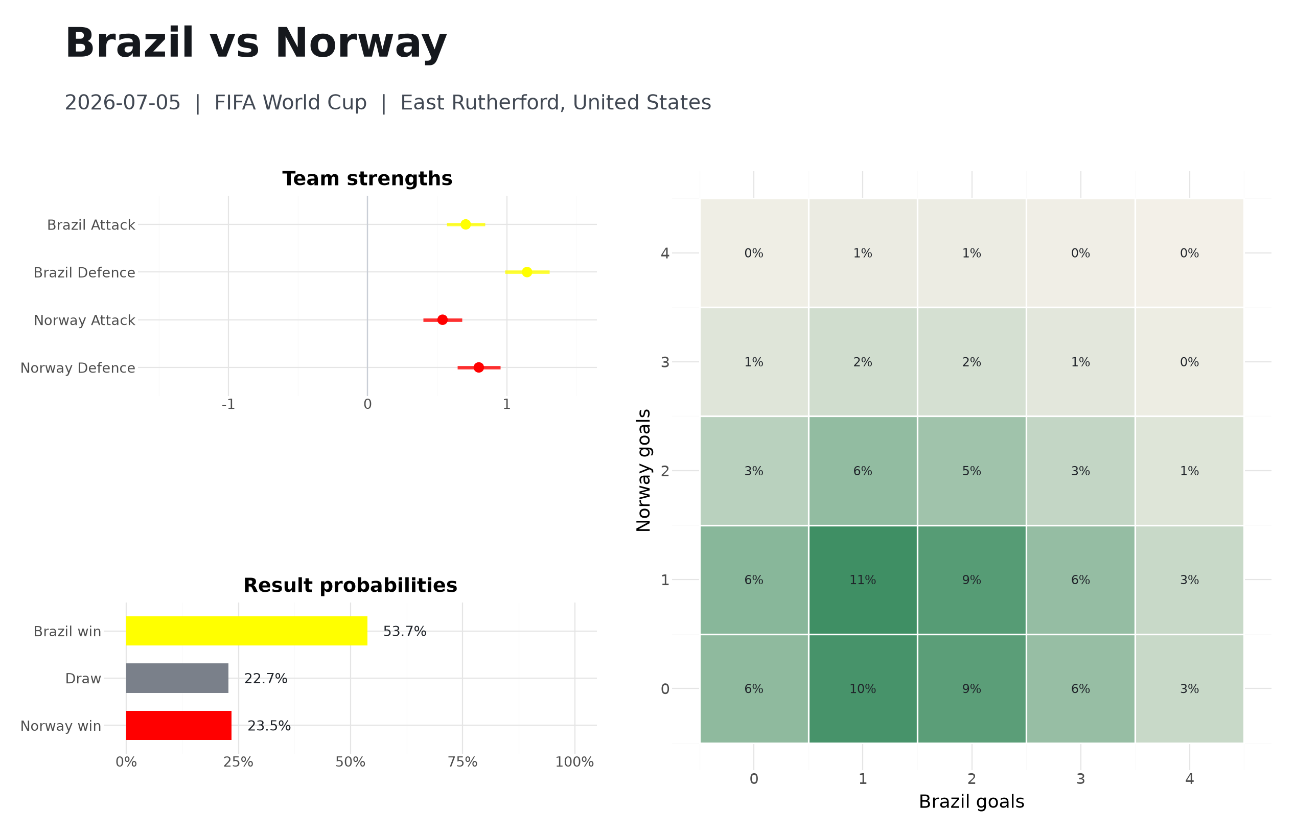
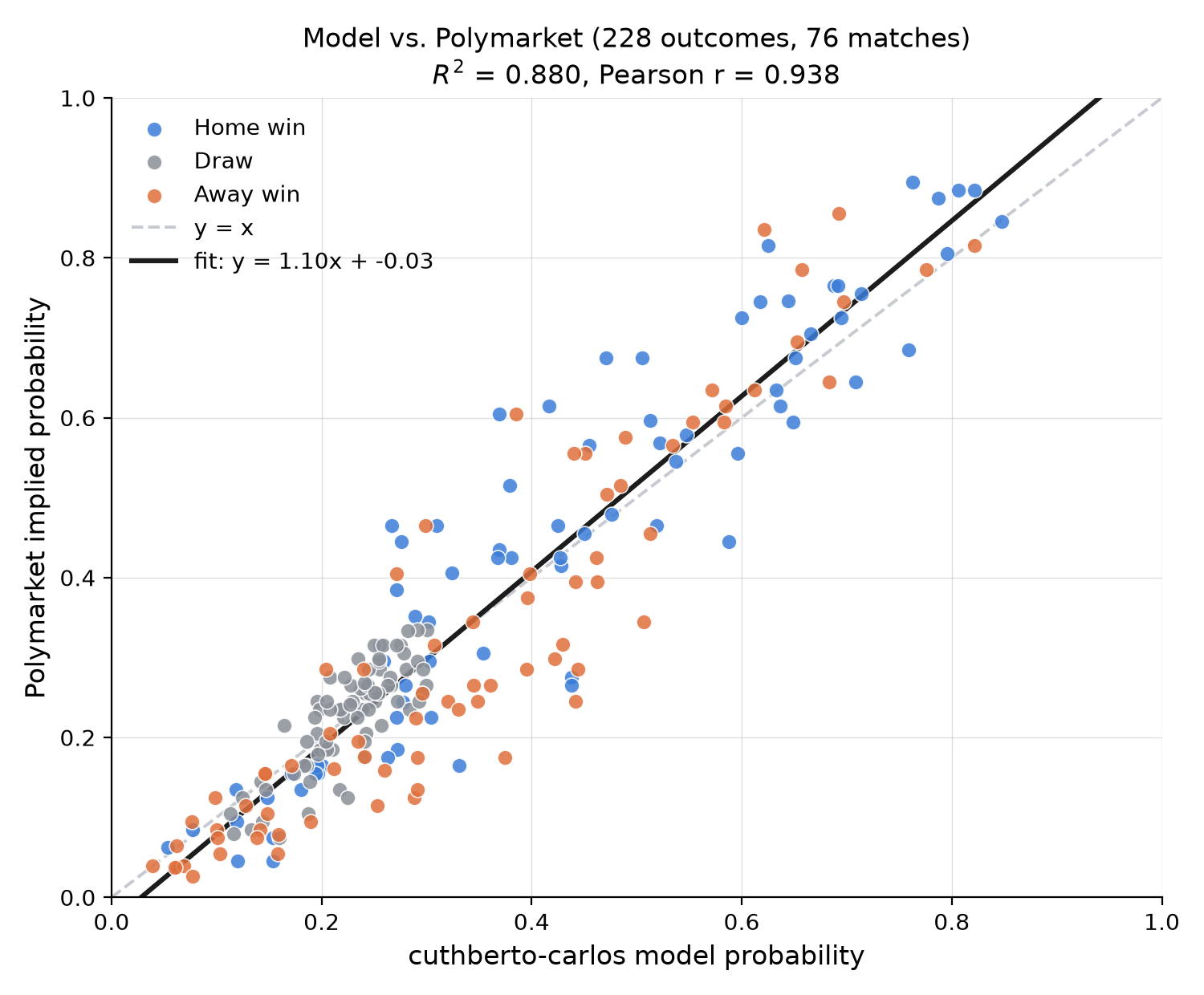
Filtered team strengths, full score grid, win/draw/loss probabilities. Checked live against Polymarket odds: \(R^2 = 0.88\), Pearson \(r = 0.94\), fit slope \(1.10\).

Roadmap & call for contributions

cuthbert: open and active.

Open an issue if you have a question, suggestion, or spotted a bug. Start or join a discussion about design/methods etc. Open a pull request. Join us on Discord.

dynestyx: concrete, documented gaps to fill.

• control_model (exogenous/control inputs): not yet implemented
• In-window smoothing and latent-path predictions: not yet supported (only predict_times ≥ max(obs_times) today)
• UKF smoothing through the cuthbert backend: not yet wired up

Concrete “where to start” points, for anyone who wants to get involved.

Thank you

• github.com/state-space-models/cuthbert
• github.com/BasisResearch/dynestyx
• Discord: come chat about state-space models

cuthbert maintainers:

Sam Duffield

Sahel Iqbal

Adrien Corenflos

dynestyx people: Dan Waxman, Dmitry Batenkov, John Feser, Andy Zane, Eli Bingham, Youssef Marzouk, Matthew E. Levine