Maximin Robust Bayesian Experimental Design

A Minimax Framework against Model Misspecification

Adrien Corenflos

Department of Statistics, University of Warwick

Co-Authors


Hany Abdulsamad
University of Amsterdam


Sahel Iqbal
Aalto University/Oxford University


Christian A. Naesseth
University of Amsterdam


Takuo Matsubara
University of Edinburgh/Sydney

Part 1: Bayesian Experimental Design

Setup

An experimenter selects a design \(\xi \in \Xi\) to infer latent parameters \(\theta \in \Theta\) from outcomes \(x \in \mathcal{X}\).

The probabilistic model:

  • Prior: \(p(\theta)\)
  • Likelihood: \(p(x \mid \theta, \xi)\)
  • Marginal: \(p(x \mid \xi) = \int p(x \mid \theta, \xi)\, p(\theta)\, \mathrm{d}\theta\)
  • Posterior: \(p(\theta \mid x, \xi) \propto p(\theta)\, p(x \mid \theta, \xi)\)

Goal: choose \(\xi^{\star}\) to learn as much about \(\theta\) as possible before the data arrives.

Expected Information Gain

A useful design is one whose data update changes our beliefs (on average) by the most.

Formally, using the logarithmic scoring rule, the Expected Information Gain (EIG) is:

\[ I(\xi) := \mathbb{E}_{p(x \mid \xi)} \!\left[ \mathbb{D}_{\mathrm{KL}}\!\left[ p(\theta \mid x, \xi) \;\middle\|\; p(\theta) \right] \right] = \mathbb{E}_{p(\theta)} \!\left[ \mathbb{D}_{\mathrm{KL}}\!\left[ p(x \mid \theta, \xi) \;\middle\|\; p(x \mid \xi) \right] \right] \]

This is Shannon’s mutual information \(I(\theta; x)\) under \(\xi\). The optimal design is \(\xi^{\star} = \arg\max_{\xi \in \Xi}\, I(\xi)\).

Decision-theoretic grounding: the EIG is the largest expected improvement in log-probability forecast achievable by running the experiment.

Part 2: The Core Problem

EIG is Fragile Under Misspecification

When the model \(p(\theta, x \mid \xi)\) is only a surrogate, \(I(\xi)\) becomes unreliable.

Why? The EIG has a nested dependence on the likelihood:

  • The posterior \(p(\theta \mid x, \xi) \propto p(\theta)\, p(x \mid \theta, \xi)\) depends on it.
  • The marginal \(p(x \mid \xi)\) defining the outer expectation also depends on it.

Under misspecification, \(I(\xi)\) may favour designs that appear informative under the assumed model but fail to deliver when confronted with reality.

The Boundary-Seeking Pathology

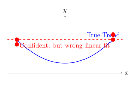
A canonical symptom: if we trust a linear model, the optimal design concentrates all samples at the boundaries of the design space.

We learn nothing about the interior, and if the model is wrong, we cannot even detect it.

Our Approach: Distributional Robustness

We do not try to specify which alternative model might hold. Instead, we protect against any deviation within an information-theoretic budget.

Goal: design experiments that perform well even if the entire data-generating distribution is perturbed within a bounded KL neighbourhood.

Part 3: Maximin Robust Bayesian Experimental Design

A Two-Player Zero-Sum Game

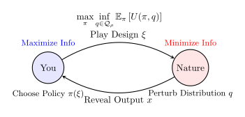
We model misspecification as a Stackelberg game between the experimenter and an adversarial nature.

  • Nature selects an adversarial joint law \(q(\theta, x \mid \xi)\) from an admissible set \(\mathcal{Q}\).
  • Experimenter counters with a stochastic design policy \(\pi \in \Pi\).

The experimenter seeks robustness by solving the maximin problem:

\[ \pi^{\star} \;:=\; \arg\max_{\pi \in \Pi} \, \inf_{q \in \mathcal{Q}} \; \mathbb{E}_{\pi}\!\left[ U(\xi, q) \right]. \]

The Payoff Function

What is the value of design \(\xi\) against an adversarial law \(q(\theta, x \mid \xi)\)?

The experimenter commits to the prior \(p(\theta)\) as a fixed reference forecast and optimizes the post-observation forecast rule. Under the log scoring rule, this yields:

\[ U(\xi, q) \;=\; \sup_{\psi_\xi} \int q(\theta, x \mid \xi)\Big[\log \psi_\xi(x)(\theta) - \log p(\theta)\Big]\,\mathrm{d}\theta\,\mathrm{d}x. \]

The supremum is attained at \(\psi_\xi^\star(x) = q(\cdot \mid x, \xi)\), giving the closed form:

\[ U(\xi, q) \;=\; \mathbb{D}_{\mathrm{KL}}\!\left[ q(\theta, x \mid \xi) \;\middle\|\; p(\theta)\, q(x \mid \xi) \right]. \]

The KL Ambiguity Set

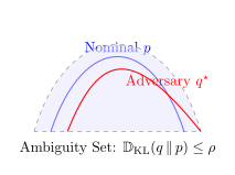
Without constraints, nature trivially sets \(\theta \perp x\) and drives the gain to zero. We constrain nature to an average KL neighbourhood of the nominal model:

\[ \mathcal{Q}_{\rho}(\pi) \;:=\; \left\{ q(\theta, x \mid \xi) \;\Big|\; \mathbb{E}_{\pi}\!\left[ \mathbb{D}_{\mathrm{KL}}\!\left[ q(\theta, x \mid \xi) \;\middle\|\; p(\theta, x \mid \xi) \right] \right] \le \rho \right\}. \]

  • \(p(\theta, x \mid \xi)\): experimenter’s nominal model, their best approximation to reality.
  • \(\rho > 0\): misspecification budget. Small \(\rho\) means mild perturbations; large \(\rho\) means strong misspecification.
  • The average constraint lets nature allocate its budget strategically, attacking the most informative designs most aggressively.

Solving the Game: Lagrangian Decomposition

The inner minimisation \(\inf_{q \in \mathcal{Q}_\rho} \mathbb{E}_\pi[U(\xi,q)]\) is solved via Lagrangian duality. The global problem decomposes into pointwise regularized problems:

\[ \inf_{q \in \mathcal{Q}_{\rho}} \mathbb{E}_{\pi}\!\left[U(\xi, q)\right] \;=\; \sup_{\beta > 0} \left\{ \mathbb{E}_{\pi}\!\left[\mathcal{J}_{\beta}(\xi)\right] - \beta\rho \right\}, \]

where \(\mathcal{J}_{\beta}(\xi)\) is the regularized pointwise utility:

\[ \mathcal{J}_{\beta}(\xi) \;:=\; \inf_{q}\, \Big\{ U(\xi, q) + \beta\, \mathbb{D}_{\mathrm{KL}}\!\left[ q(\theta, x \mid \xi) \;\middle\|\; p(\theta, x \mid \xi) \right] \Big\}. \]

The dual parameter \(\beta\) (or equivalently \(\rho\)) is a robustness knob: larger \(\beta\) penalizes deviations more, reflecting greater trust in the nominal model.

Main Result: Robust EIG = Sibson’s \(\alpha\)-MI

Proposition. For \(\beta > 0\), let \(\alpha := \beta/(1+\beta) \in (0,1)\). Then \(\mathcal{J}_\beta(\xi)\) admits the closed form:

\[ \begin{aligned} \mathcal{J}_{\beta}(\xi) \;=\; \inf_{\nu}\, \mathbb{D}_{\alpha}\!\left[ p(\theta, x \mid \xi) \;\middle\|\; p(\theta)\,\nu(x \mid \xi) \right] \;&=\; \mathbb{D}_{\alpha}\!\left[ p(\theta, x \mid \xi) \;\middle\|\; p(\theta)\,p_{\alpha}(x \mid \xi) \right] \\ &=:\, I^{S}_{\alpha}(\theta; x)(\xi), \end{aligned} \]

where \(\mathbb{D}_{\alpha}\) is Rényi’s divergence of order \(\alpha\), and the \(\alpha\)-tilted marginal is:

\[ p_{\alpha}(x \mid \xi) \;\propto\; \left[\mathbb{E}_{p(\theta)}\!\left[ p(x \mid \theta, \xi)^{\alpha} \right]\right]^{1/\alpha}. \]

The quantity \(I^{S}_{\alpha}(\theta; x)(\xi)\) is Sibson’s \(\alpha\)-mutual information: a known but rarely used information measure, here emerging from first principles as the robust expected information gain.

The order \(\alpha\) is the dual variable associated with the KL radius \(\rho\), encoding the experimenter’s confidence in the nominal model.

The Worst-Case Posterior: \(\alpha\)-Tilted Inference

Corollary. The adversarial joint law that achieves the infimum in the previous result is a geometric mixture. Its implied posterior is:

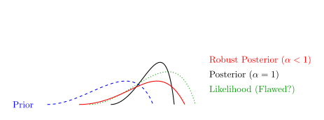
\[ q^{\star}(\theta \mid x, \xi) \;\propto\; p(\theta)\, p(x \mid \theta, \xi)^{\alpha}. \]

Acting consistently with the adversarial assumption requires tempering the likelihood with \(\alpha \in (0,1)\). This is the update rule of generalized Bayesian inference under misspecification.

Interpreting \(\alpha\)

Robustness is governed by the monotonicity of Sibson’s \(\alpha\)-MI in \(\alpha\):

  • \(\alpha \to 1\): the ambiguity set contracts; adversarial influence vanishes; \(I^{S}_{\alpha} \to I\) (standard EIG).

  • \(\alpha \to 0\): nature exerts maximal influence; \(\sup_{\xi} I^{S}_{\alpha}(\theta; x)(\xi) \to 0\), no design can guarantee information gain against an unconstrained adversary.

  • \(\alpha \in (0,1)\): a principled middle ground. The design favours outcomes whose information gain is stable under perturbation, not just high under the nominal model.

Like the choice of prior \(p(\theta)\), \(\alpha\) is a subjective modeling variable expressing the experimenter’s confidence in \(p(\theta, x \mid \xi)\).

Risk-Sensitive Form: Rényi Divergence as Conditional Info Gain

Proposition. Sibson’s \(\alpha\)-MI admits the risk-sensitive representation:

\[ I^{S}_{\alpha}(\theta; x)(\xi) \;=\; \frac{\alpha}{\alpha - 1} \log\,\mathbb{E}_{p(x \mid \xi)}\!\left[\exp\!\left\{\frac{\alpha - 1}{\alpha}\, G_{\alpha}(x, \xi)\right\}\right], \]

where \(G_{\alpha}(x, \xi) := \mathbb{D}_{\alpha}\!\left[ p(\theta \mid x, \xi) \;\middle\|\; p(\theta) \right]\) is the per-outcome Rényi gain.

This mirrors the interpretation of the EIG as \(\mathbb{E}_{p(x|\xi)}\!\left[\mathbb{D}_{\mathrm{KL}}\!\left[ p(\theta|x,\xi) \;\middle\|\; p(\theta) \right]\right]\), but:

  • the utility is a Rényi divergence (not KL) between posterior and prior, and
  • the aggregation is a risk-sensitive exponential average (not an arithmetic mean).

Second-order expansion around \(\alpha = 1\):

\[ I^{S}_{\alpha}(\theta; x)(\xi) \;\approx\; I(\xi) \;+\; \frac{\alpha - 1}{2}\, \operatorname{Var}_{p(\theta, x \mid \xi)}\!\left[\log\frac{p(\theta \mid x, \xi)}{p(\theta)}\right]. \]

For \(\alpha < 1\): penalizes variance of the information gain across design-outcome pairs, favouring designs that are reliably informative.

Part 4: Estimation & PAC-Bayesian Policies

The Computational Challenge

Sibson’s \(\alpha\)-MI provides a robust theoretical objective, but it is intractable to compute exactly.

It requires computing nested expectations. We employ a Nested Monte Carlo (NMC) estimator \(\tilde{I}^S_\alpha(\xi)\):

\[ \tilde{I}^{S}_{\alpha}(\xi) \approx \frac{\alpha}{\alpha-1} \log \left( \frac{1}{N} \sum_{i=1}^N \left[ \frac{1}{M} \sum_{j=1}^M w(x^{(i)}, \theta^{(i, j)}, \xi)^{\alpha} \right]^{1/\alpha} \right) \]

The Catch: Because of the nonlinear \(\log\) and power functions, this empirical estimator is biased and has high variance.

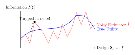
The Danger of Noisy Optimization

Plugging a biased, noisy estimator directly into gradient descent is unstable.

  • Exploitation: Continual optimization will seek out regions where the Monte Carlo noise is favourably biased.
  • Overfitting: The deterministic design overfits to the finite samples.

We need an optimization procedure that acknowledges the estimator’s flaws.

The Need for Stochastic Policies

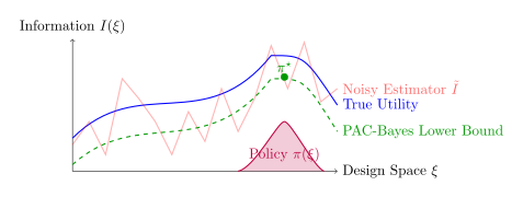
Instead of searching for a single best design \(\xi^*\), we shift to a PAC-Bayesian framework.

  • We view design selection as a continuous bandit problem.
  • We search for a stochastic design policy \(\pi(\xi)\) (a distribution over designs).
  • Goal: Find a policy that guarantees high performance with high probability (Probably Approximately Correct) over the randomness of the data estimator.

The PAC-Bayes Guarantee

We can prove uniform concentration bounds for our estimator. This leads to a PAC-Bayes lower bound.

With high probability, the following holds simultaneously for all policies \(\pi \in \Pi\):

\[ \mathbb{E}_{\pi} \big[I_{\alpha}^{S}(\xi) \big] \ge \mathbb{E}_{\pi} \big[ \tilde{I}_{\alpha}^{S}(\xi) \big] - \frac{\lambda L_{f}^{2} C_{h}^{2}}{2N} - \frac{\text{KL}(\pi \| \pi_{0}) + \log(1/\delta)}{\lambda} \]

  • \(\mathbb{E}_{\pi} \big[ \tilde{I}_{\alpha}^{S}(\xi) \big]\): Empirical performance on the noisy surrogate.
  • \(\text{KL}(\pi \| \pi_{0})\): Complexity penalty restricting divergence from a safe base policy \(\pi_{0}\).

Tractable Optimization

We cannot directly optimize the true information \(I_{\alpha}^{S}\), but we can maximize its PAC-Bayesian lower bound!

Dropping constants independent of \(\pi\) gives \(\pi^{\star} = \arg\max_{\pi \in \Pi} \, \left\{ \mathbb{E}_{\pi} \big[ \tilde{I}_{\alpha}^{S}(\xi) \big] - \frac{\text{KL}(\pi \| \pi_{0})}{\lambda} \right\}.\)

\[ \pi^{\star} = \arg\max_{\pi \in \Pi} \, \left\{ \mathbb{E}_{\pi} \big[ \tilde{I}_{\alpha}^{S}(\xi) \big] - \frac{\text{KL}(\pi \| \pi_{0})}{\lambda} \right\} \]

The result is an closed-form Gibbs policy: \(\pi^{\star}(\xi) \propto \pi_{0}(\xi) \exp \left\{ \lambda \tilde{I}_{\alpha}^{S}(\xi) \right\}\).

Empirical Evidence

Realized Information Gain

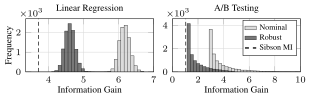
We compare designs selected by the nominal (\(\alpha = 1\)) and robust (\(\alpha < 1\)) objectives, evaluated against the true (misspecified) data-generating process.

  • Nominal: reports high subjective gain but this is self-referential, measured under the wrong model.
  • Robust: reports a lower, but honest gain under both the nominal and the true process.

Posterior Coverage

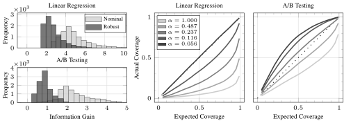
Does the posterior reliably contain the true parameter?

  • Nominal posteriors: systematic overconfidence.
  • Robust posteriors: conservative, can be calibrated.

Optimizing the design amplifies the benefit: robust designs actively seek outcomes that keep coverage honest.

Conclusion

Summary

  1. The framework: cast robust BED as a max-min Stackelberg game with a KL ambiguity set: distributional robustness via DRO.

  2. The objective: the game yields Sibson’s \(\alpha\)-mutual information as the robust EIG, with \(\alpha \in (0,1)\) controlling the conservatism of the design.

  3. The inference rule: the worst-case adversary dictates the \(\alpha\)-tilted posterior \(q^\star(\theta \mid x,\xi) \propto p(\theta)\,p(x \mid \theta,\xi)^\alpha\). Robust design and generalized Bayesian inference emerge jointly.

  4. The geometry: Rényi divergence is the natural per-outcome information metric; Sibson’s \(\alpha\)-MI is its risk-sensitive aggregation, penalizing variance of information gain for \(\alpha < 1\).


Thank you!    Preprint: arxiv.org/abs/2603.14094