Maximin Robust Bayesian Experimental Design

A Minimax Framework against Model Misspecification

Adrien Corenflos

Department of Statistics, University of Warwick

Co-Authors

Hany Abdulsamad
University of Amsterdam

Sahel Iqbal
Aalto University/Oxford University

Christian A. Naesseth
University of Amsterdam

Takuo Matsubara
University of Edinburgh/Sydney

Overview

• Part 1: Introduction to Bayesian Experimental Design.
• Part 2: The Core Problem: Fragility to model misspecification.
• Part 3: Robust BED: A max-min game against an adversarial nature.
• Part 4: Optimization: PAC-Bayesian policies for noisy estimators.
• Part 5: Numerical Evaluation in Linear Regression and A/B Testing.

Part 1: Intuition of Bayesian Experimental Design

The Reality of Data Collection

Data doesn’t just magically appear. Gathering data in the real world is expensive, time-consuming, and potentially risky.

We have to collect it, and we have to collect it efficiently.

The Experimental Design Loop

Instead of a static dataset, we actively choose experimental conditions \(\xi\).

Why Bayesian Experimental Design?

Frequentist Design typically optimizes for the best-case or average-case variance of an estimator around a fixed “true” parameter \(\theta_{\text{true}}\).

Bayesian Design explicitly models our uncertainty over \(\theta\) before the experiment.

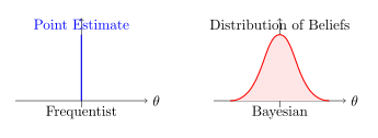
We design experiments to maximally shrink this entire distribution.

Quantifying Uncertainty

How do we rigorously measure the “volume” of our uncertainty?

Shannon Entropy measures the unpredictability of a distribution \(p(\theta)\): \[ H(p) = - \mathbb{E}_{p(\theta)} [\log p(\theta)] \]

When we observe data \(x\), we update our belief from the prior \(p(\theta)\) to the posterior \(p(\theta \mid x, \xi)\).

The Kullback-Leibler (KL) divergence is the relative entropy that quantifies the information gained by this update: \[ \mathbb{D}_{\mathrm{KL}} \left[ p(\theta \mid x, \xi) \,\|\, p(\theta) \right] = \mathbb{E}_{p(\theta \mid x, \xi)} \left[ \log \frac{p(\theta \mid x, \xi)}{p(\theta)} \right] \]

Measuring Information Gain

We want our experiment to reduce our uncertainty about \(\theta\) as much as possible on average.

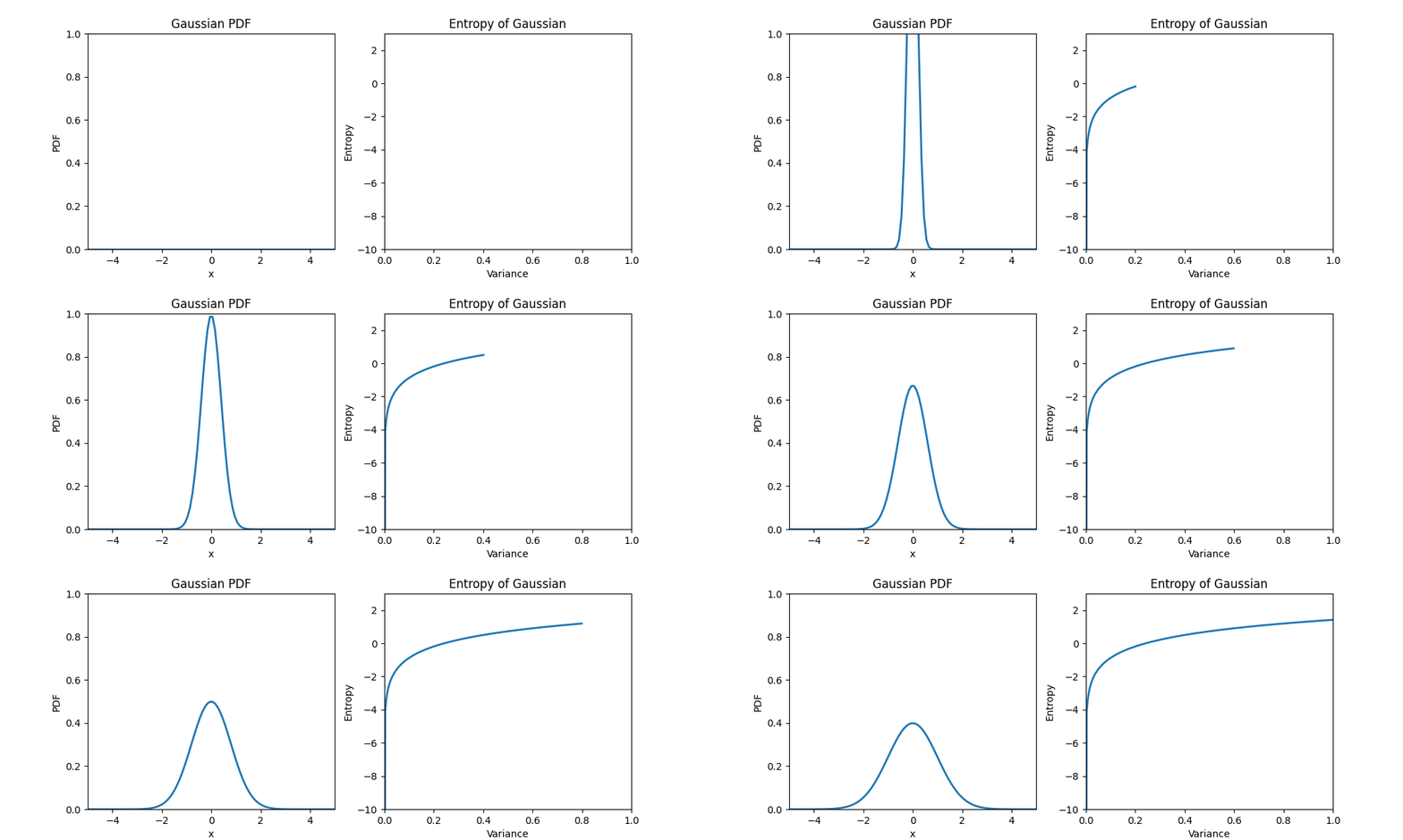
The Expected Information Gain (EIG) measures this expected shrinkage before we collect the data: \[ I(\xi) = \mathbb{E}_{p(x \mid \xi)} \left[ \mathbb{D}_{\mathrm{KL}} \left[ p(\theta \mid x, \xi) \,\|\, p(\theta) \right] \right] \]

Part 2: The Core Problem & Types of Robustness

The Fragility of the “Ideal” Model

Classical and Bayesian optimal designs share a critical flaw: they take the model literally.

The Model: The Perfect World

The Reality: A Misspecified World

The Boundary-Seeking Pathology

If we trust a linear model, the optimal design places all samples at the boundaries to maximize variance.

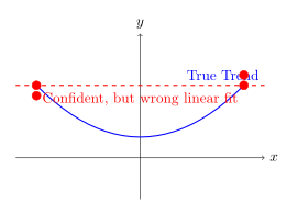
We learn nothing about the middle!

Different Concepts of Robustness

Before we propose a solution, let’s distinguish our approach from other types of robustness.

1. Robust Statistics (Against Outliers)

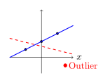
Goal: Ensure inference isn’t broken by a few bad data points. (Not our focus here).

Different Concepts of Robustness (cont.)

2. Distributional Robustness (Our Approach)

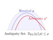
Goal: Perform well even if the entire data-generating distribution is perturbed within a budget.

Part 3: Maximin Robust Bayesian Experimental Design

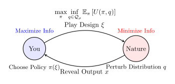
Robustification: A Max-Min Game

Instead of trusting the nominal model \(p(x \mid \theta, \xi)\), we assume nature is adversarial.

We frame the design problem as a two-player zero-sum game:

The Ambiguity Set

Nature isn’t allowed to do whatever it wants; it is bound by an information-theoretic budget.

We restrict nature to an Ambiguity Set \(\mathcal{Q}_{\rho}\):

\[ \mathcal{Q}_{\rho}(\pi) := \left\{ q(\cdot \mid \xi) \, \Big| \, \mathbb{E}_{\pi} \left[ \mathbb{D}_{\mathrm{KL}} \left[ q(\cdot \mid \xi) \,\|\, p(\cdot \mid \xi) \right] \right] \le \rho \right\} \]

• \(p(\cdot \mid \xi)\) is our nominal (assumed) joint model.
• \(\rho\) is the budget. Small \(\rho\) means mild misspecification; large \(\rho\) means misspecification.

Solving the Game

How do we solve this adversarial game?

By introducing Lagrangian multipliers and solving the inner infimum, the optimal adversarial distribution \(q^\star\) yields a simple result for our inferences.

The worst-case posterior becomes the \(\alpha\)-tilted posterior:

\[ q^\star(\theta \mid x, \xi) \propto p(\theta) \left[ p(x \mid \theta, \xi) \right]^\alpha \]

where \(\alpha \in (0, 1)\) is uniquely determined by the ambiguity radius \(\rho\).

Tempering the Likelihood

What does the \(\alpha\)-tilted posterior tell us?

\[ q^\star(\theta \mid x, \xi) \propto p(\theta) \left[ p(x \mid \theta, \xi) \right]^\alpha \]

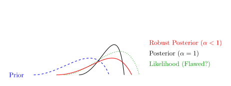
• To be robust against misspecification, we must temper (downweight) our likelihood.
• This intuitively guards against overconfidence in any single observation generated by a potentially flawed model.

Why Does This Work for Statisticians?

By framing robustness through an adversarial lens, we recover a rigorous justification for fractional posteriors (generalized Bayesian inference) in experimental design.

• Standard BED: Maximizes information under the strong assumption the model is perfectly true.
• Robust BED (\(\alpha < 1\)): Maximizes information while enforcing a degree of skepticism about the assumed data-generating process.

The Robust Objective: Sibson’s \(\alpha\)-MI

When we plug the optimal adversary back into our game, we no longer need to simulate the adversary.

The robust expected information gain evaluates exactly to a known, but rarely used, information measure: Sibson’s \(\alpha\)-Mutual Information.

\[ I^S_\alpha(\theta; x)(\xi) = \mathbb{D}_{\alpha} \left[ p(\theta, x \mid \xi) \,\|\, p(\theta) \, p_{\alpha}(x \mid \xi) \right] \]

where \(\mathbb{D}_{\alpha}\) is the Rényi divergence of order \(\alpha\), defined for distributions \(p\) and \(q\) as: \[ \mathbb{D}_{\alpha} \left[ p \,\|\, q \right] = \frac{1}{\alpha - 1} \log \int p(z)^\alpha q(z)^{1-\alpha} \mathrm{d}z \]

Interpreting Sibson’s \(\alpha\)-MI

\[ I^S_\alpha(\theta; x)(\xi) = \mathbb{D}_{\alpha} \left[ p(\theta, x \mid \xi) \,\|\, p(\theta) \, p_{\alpha}(x \mid \xi) \right] \]

• As \(\alpha \to 1\) (no misspecification allowed): We recover standard Expected Information Gain (EIG).
• As \(\alpha \to 0\) (infinite adversary budget): The maximum achievable information gain diminishes to zero. The design avoids over-committing and seeks to explore uniformly.
• The Sweet Spot: Choosing an \(\alpha \in (0,1)\) naturally leads to more space-filling, less boundary-seeking designs. They gather evidence to check the model, rather than just exploiting it blindly.

\[ \mathbb{D}_{\alpha} \left[ p \,\|\, q \right] = \frac{1}{\alpha - 1} \log \int p(z)^\alpha q(z)^{1-\alpha} \mathrm{d}z \]

Part 4: Estimation & PAC-Bayesian Policies

The Computational Challenge

Sibson’s \(\alpha\)-MI provides a robust theoretical objective, but it is intractable to compute exactly.

It requires computing nested expectations. We employ a Nested Monte Carlo (NMC) estimator \(\tilde{I}^S_\alpha(\xi)\):

\[ \tilde{I}^{S}_{\alpha}(\xi) \approx \frac{\alpha}{\alpha-1} \log \left( \frac{1}{N} \sum_{i=1}^N \left[ \frac{1}{M} \sum_{j=1}^M w(x^{(i)}, \theta^{(i, j)}, \xi)^{\alpha} \right]^{1/\alpha} \right) \]

The Catch: Because of the nonlinear \(\log\) and power functions, this empirical estimator is biased and has high variance.

The Danger of Noisy Optimization

Plugging a biased, noisy estimator directly into gradient descent is unstable.

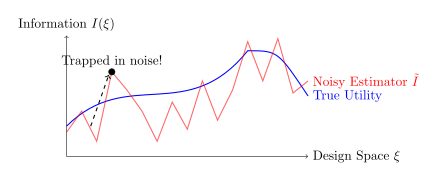
• Exploitation: Continual optimization will seek out regions where the Monte Carlo noise is favorably biased.
• Overfitting: The deterministic design overfits to the finite samples.

We need an optimization procedure that acknowledges the estimator’s flaws.

The Need for Stochastic Policies

Instead of searching for a single best design \(\xi^*\), we shift to a PAC-Bayesian framework.

• We view design selection as a continuous bandit problem.
• We search for a stochastic design policy \(\pi(\xi)\) (a distribution over designs).
• Goal: Find a policy that guarantees high performance with high probability (Probably Approximately Correct) over the randomness of the data estimator.

The PAC-Bayes Guarantee

We can prove uniform concentration bounds for our estimator. This leads to a PAC-Bayes lower bound.

With high probability, the following holds simultaneously for all policies \(\pi \in \Pi\):

\[ \mathbb{E}_{\pi} \big[I_{\alpha}^{S}(\xi) \big] \ge \mathbb{E}_{\pi} \big[ \tilde{I}_{\alpha}^{S}(\xi) \big] - \frac{\lambda L_{f}^{2} C_{h}^{2}}{2N} - \frac{\text{KL}(\pi \| \pi_{0}) + \log(1/\delta)}{\lambda} \]

• \(\mathbb{E}_{\pi} \big[ \tilde{I}_{\alpha}^{S}(\xi) \big]\): Empirical performance on the noisy surrogate.
• \(\text{KL}(\pi \| \pi_{0})\): Complexity penalty restricting divergence from a safe base policy \(\pi_{0}\).

Tractable Optimization

We cannot directly optimize the true information \(I_{\alpha}^{S}\), but we can maximize its PAC-Bayesian lower bound!

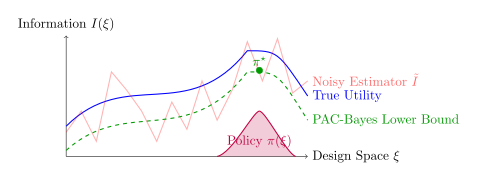
Dropping constants independent of \(\pi\) gives \(\pi^{\star} = \arg\max_{\pi \in \Pi} \, \left\{ \mathbb{E}_{\pi} \big[ \tilde{I}_{\alpha}^{S}(\xi) \big] - \frac{\text{KL}(\pi \| \pi_{0})}{\lambda} \right\}.\)

\[ \pi^{\star} = \arg\max_{\pi \in \Pi} \, \left\{ \mathbb{E}_{\pi} \big[ \tilde{I}_{\alpha}^{S}(\xi) \big] - \frac{\text{KL}(\pi \| \pi_{0})}{\lambda} \right\} \]

The result is an closed-form Gibbs policy: \(\pi^{\star}(\xi) \propto \pi_{0}(\xi) \exp \left\{ \lambda \tilde{I}_{\alpha}^{S}(\xi) \right\}\).

Part 5: Empirical Evidence

Experimental Setup

We evaluated our framework on two canonical settings subjected to misspecification:

1. Linear Regression:
   • A high-dimensional design search with misspecified heteroskedastic noise.
2. A/B Testing:
   • Allocating samples between treatment arms where the true base conversion rates violate prior assumptions.

Realized Information Gain

We compare the realized information gain under nominal and robust formulations using optimal designs.

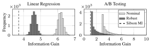
• The nominal experimenter sees high “subjective” information gain, but this measurement is self-referential because the utility relies on the misspecified likelihood.
• The robust experimenter yields a lower, but more realistic, information gain that does not over-promise on inference accuracy.

Posterior Coverage

Coverage measures calibration: Does the posterior contain the truth?

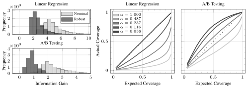
• Nominal Posteriors: Curves lie below the diagonal (overconfident, systematic underdelivery).
• Robust Posteriors: Curves lie above the diagonal (conservative, overcoverage).
• Optimizing the design amplifies this necessary conservativeness.

PAC-Bayes Design Optimality

Evaluating realized regret and design optimality of a PAC-Bayes policy vs. Naive optimization (Gradient Descent / Enumeration).

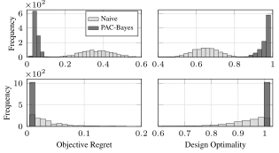
• Naive optimizers incur higher and more variable regret, getting trapped by estimator noise.
• The PAC-Bayes policy concentrates near the optimum and achieves lower regret.

Conclusion

Summary

1. Robust Inference: Under misspecification, standard BED yields severe undercoverage. The \(\alpha\)-tilted posterior yields conservative, well-calibrated coverage.
2. Optimal Robust Allocation: Minimizing Sibson’s \(\alpha\)-MI actively forces sampling allocations away from boundary edge cases, hedging against extreme prior-data conflicts.
3. PAC-Bayes Superiority: Optimizing stochastic policies via PAC-Bayes achieves significantly lower regret than naive deterministic optimization.

Takeaway

Robust Bayesian Experimental Design unifies adversarial robustness and generalized Bayesian learning, providing a rigorous and scalable pathway for designing experiments you can trust in the real world.

Grazie per l’attenzione!

https://arxiv.org/abs/2603.14094