Computing importance weights for Markov chain Monte Carlo via couplings: an application to f-divergence diagnostics
Department of Statistics, University of Warwick
Joint work with Hai-Dang Dau

College of Computing and Data Science, Nanyang Technological University
Motivation: MCMC
MCMC is used to compute expectations \(\pi(\varphi) = \mathbb{E}_{\pi}[\varphi(X)]\) when sampling from a target \(\pi\) is impossible.
Method:
- Design a kernel \(K\) with invariant distribution \(\pi\): i.e., \(\pi\, K = \pi\).
- Simulate \(X_{t+1} \sim K(X_t, \cdot)\), with \(\mathcal{L}(X_t) \to \pi\) as \(t \to \infty\).
- Use time averages to approximate expectations: \[\begin{equation} \pi(\varphi) \approx \frac{1}{T-B+1} \sum_{t=B}^T \varphi(X_t) \end{equation}\]
Nagging Question: “are we there yet?”
Standard diagnostics:
- Gelman-Rubin (\(\hat{R}\)): Compares variance within and between \(2N\) parallel chains. A variance ratio \(\hat{R} \approx 1\) suggests convergence.
- Effective Sample Size (ESS): Estimates the number of independent samples equivalent to the MCMC output for a given function \(\varphi\). \[\begin{equation} \text{ESS} = \frac{T}{1 + 2 \sum_{k=1}^T \text{Corr}(\varphi(X_0), \varphi(X_k))} \end{equation}\]
Limitations of Standard Diagnostics
The Gelman-Rubin diagnostic (Gelman and Rubin 1992) and ESS have a key limitation:
They are function-specific.
- A chain might have a good ESS for \(\mathbb{E}[X]\) but a terrible one for \(\mathbb{E}[X^2]\).
- We get a partial picture of convergence, tied to specific test functions \(\varphi\).
Wouldn’t it be better to diagnose the convergence of the distribution of the chain itself?
Distribution-based Diagnostics
Theoretical convergence is measured by statistical distances between the chain’s distribution \(\mu_t\) and the target \(\pi\).
- Total Variation Distance: \(\|\mu_t - \pi\|_{\text{TV}}\)
- Wasserstein Distance: \(W_p(\mu_t, \pi)\)
Biswas, Jacob, and Vanetti (2019) provide computable upper bounds on these distances using coupled chains.
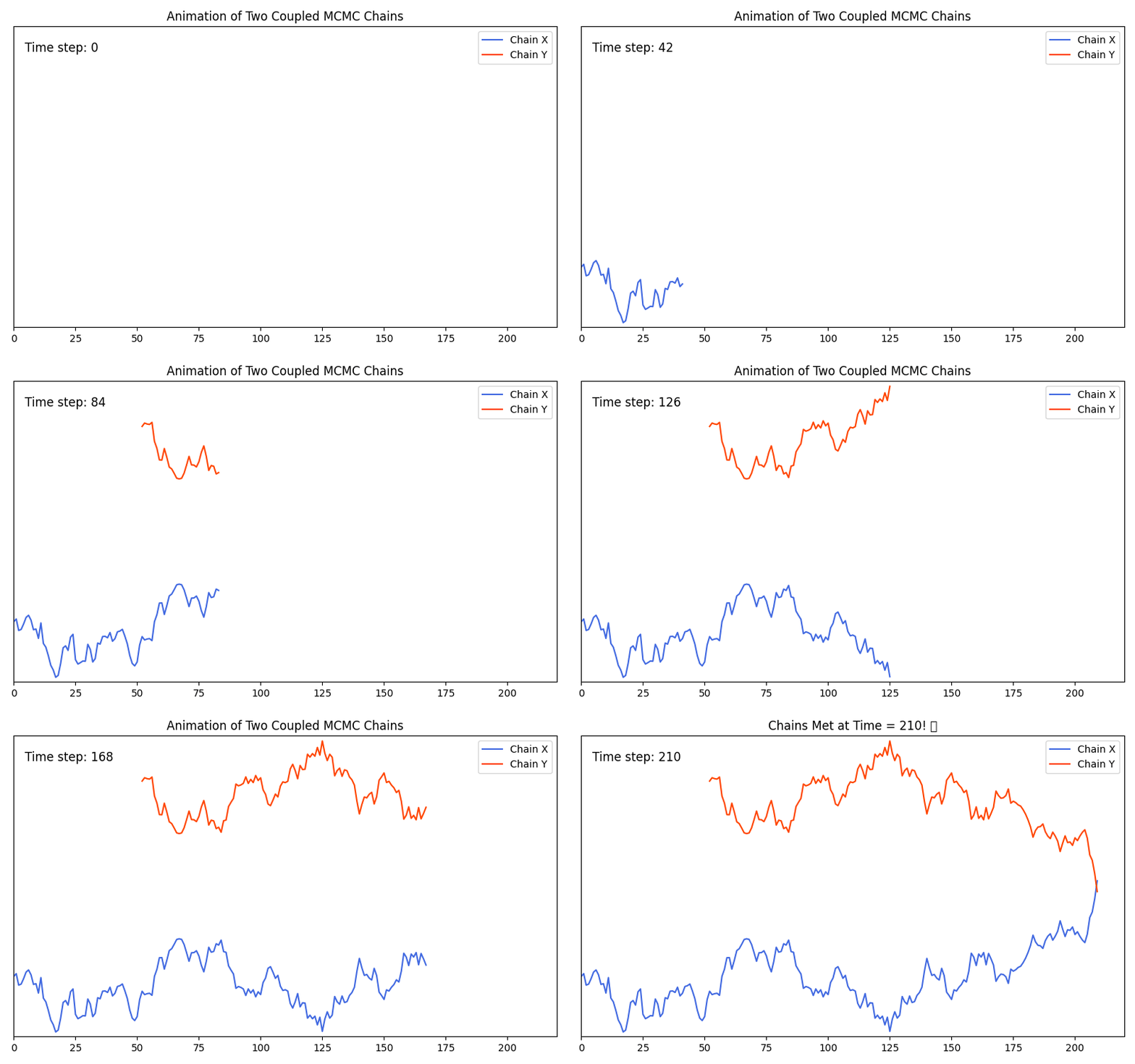
A coupling runs two chains \((X_t, Y_t)\) jointly to make them meet:
If \(X_{t+L} \sim \pi\) and \(Y_{t} \sim \mu_t\), then the meeting time \(\frac{\tau - t -L}{L}\) upper bounds \(\|\mu_t - \pi\|_{\text{TV}}\) on average.
Distribution-based Diagnostics
The independent Metropolis-Hastings case
For a target \(\pi\) and proposal \(q\), the independent Metropolis-Hastings (MH) algorithm iterates:
- Propose \(X' \sim q(\cdot)\)
- Accept \(X'\) with probability \(\alpha = 1 \wedge \tfrac{\pi(X') / q(X')}{\pi(X) / q(X)}\)
To couple two independent MH chains \((X_t, Y_t)\), we can use the same proposal \(X' \sim q(\cdot)\) for both chains at each step:
- Propose \(X' \sim q(\cdot)\)
- Compute acceptance probabilities \(\alpha_X\) and \(\alpha_Y\) for \(X_t\) and \(Y_t\) respectively.
- Draw a unique uniform random variable \(U \sim \text{Uniform}(0,1)\)
- If \(U < \alpha_X\), accept for \(X_t\); if \(U < \alpha_Y\), accept for \(Y_t\).
- If both chains accept the same proposal, they meet: \(X_{t+1} = Y_{t+1} = X'\).
Limitations of TV/Wasserstein Bounds
Practical Challenges:
- Portability: I can’t use \(\|\mu_t - \pi\|_{\text{TV}} < 0.05\) to improve my estimates of \(\mathbb{E}_\pi[\varphi(X)]\) directly.
- Lag requirement: The method requires a second chain started from a “converged” state \(Y_{t-L}\), for adaptive \(L\).
We seek a diagnostic that is:
- Distributional
- Usable
- Lag-free
Background: \(f\)-divergences
Let \(f:[0, \infty) \to \mathbb{R}\) be a convex function with \(f(1)=0\). \[\begin{equation} D_f(\pi \| \mu) = \int \mu(\mathrm{d} x) f\left( \frac{\mathrm{d}\pi}{\mathrm{d}\mu}(x) \right) \end{equation}\]
This family includes many famous divergences:
- Kullback-Leibler: \(f(t) = t \log t\)
- Total Variation: \(f(t) = |t-1|/2\)
- \(\chi^2\)-divergence: \(f(t) = (t-1)^2\)
- Hellinger distance: \(f(t) = (\sqrt{t}-1)^2\)
\(f\)-divergences for Weighted Samples
Consider two discrete measures:
- Target: \(\pi_{2N} = \sum_{n=1}^{2N} W^n \delta_{X^n}\)
- Reference: \(\mu_{2N} = \frac{1}{2N} \sum_{n=1}^{2N} \delta_{X^n}\)
The \(f\)-divergence between them is simple to compute: \[\begin{equation} D_f(\pi_{2N} \| \mu_{2N}) = \frac{1}{2N} \sum_{n=1}^{2N} f(2N W^n) \end{equation}\]
Link between \(\chi^2\)-divergences and ESS
For the \(\chi^2\)-divergence (\(f(t)=(t-1)^2\)), this becomes: \[\begin{equation} \chi^2(\pi_{2N} \| \mu_{2N}) = 2N \sum_{n=1}^{2N} (W^n)^2 - 1 \end{equation}\] This is directly related to the Effective Sample Size (ESS) for importance sampling: \[\begin{equation} \text{ESS}(W^{1:2N}) = \frac{1}{\sum (W^n)^2} = \frac{2N}{\chi^2+1} \end{equation}\]
The Ideal Scenario
Imagine we knew the density ratio \(\psi_t(x) = \frac{\mathrm{d}\pi}{\mathrm{d}\mu_t}(x)\). Given samples \(X_t^n \sim \mu_t\), we could:
- Get ideal estimates of \(\pi\) via importance sampling: \[\begin{equation} \pi(\varphi) \approx \sum_{n=1}^{2N} W_t^n \varphi(X_t^n), \quad \text{where } W_t^n \propto \psi_t(X_t^n) \end{equation}\]
- Compute any \(f\)-divergence \(D_f(\pi \| \mu_t)\), which only depends on this ratio \[\begin{equation} D_f(\pi \| \mu_t) = \mathbb{E}_{\mu_t}\left[f\left(\psi_t(X)\right)\right] \end{equation}\]
Of course, \(\psi_t(x)\) is intractable. But what if we could approximate it?
Importance Weights from MCMC Paths
If we look at the path \(X_{0:t}\) at stationarity vs. initialization, we have:
\[\begin{align*} \mathbb{P}_\pi(X_{0:t}) &= \pi(X_0) \prod_{s=1}^t K(X_{s-1}, X_s)\\ \mathbb{P}_{\mu_0}(X_{0:t}) &= \mu_0(X_0) \prod_{s=1}^t K(X_{s-1}, X_s) \end{align*}\]
The likelihood ratio over the entire path simplifies:
\[ \frac{\mathbb{P}_\pi(X_{0:t})}{\mathbb{P}_{\mu_0}(X_{0:t})} = \frac{\pi(X_0) \prod_{s=1}^t K(X_{s-1}, X_s)}{\mu_0(X_0) \prod_{s=1}^t K(X_{s-1}, X_s)} = \frac{\pi(X_0)}{\mu_0(X_0)} = w_0 \]
By choosing a test function that only keeps the \(t\)-th component (i.e., \(h(X_{0:t}) = h(X_t)\)), \(w_0\) remains a valid weight for time \(t\).
A Naive (and flawed) Approach
Based on this path-space identity, we define a simple diagnostic method:
- Start \(2N\) chains from \(X_0^n \sim \mu_0\).
- Compute initial weights \(w_0^n = \frac{\pi(X_0^n)}{\mu_0(X_0^n)}\) and normalize to \(W_0^n\).
- Run the chains: \(X_t^n \sim K^t(X_0^n, \cdot)\).
- Use the initial weights \(W_0^n\) for the samples \(X_t^n\).
Problem: This gives a consistent estimator, but the diagnostic \(\frac{1}{2N}\sum f(2N W_0^n)\) is static. It ignores all mixing done by the kernel.
We need weights that evolve.
This talk
A novel “weight harmonization” scheme for parallel MCMC chains that produces a consistent, computable approximation of the importance weights \(\psi_t(X_t^n)\).
A general method to use these weights to get online upper bounds on any \(f\)-divergence, including KL, \(\chi^2\), Hellinger, and TV distance.
The resulting diagnostic is guaranteed to improve over time and requires no lag or warm-up.
From Weights to Diagnostics
Consistency of empirical diagnostics (Theorem 1):
If we have a “good” set of weights \(W_t^{1:M}\) for our MCMC samples \(X_t^{1:M} \sim \mu_t\) (i.e., \(\sum W_t^m \delta_{X_t^m}\) is a consistent estimator of \(\pi\)), then:
\[\begin{equation} \mathbb{P}\left( \frac{1}{M}\sum_{m=1}^{M} f(M W_t^m) \le D_f(\pi \| \mu_t) - \varepsilon \right) \to 0 \quad \text{as } M \to \infty \end{equation}\]
So, if we can generate “good” weights \(W_t^m\) at each MCMC step \(t\), we can track the convergence of the chain’s distribution.
The Key Intuition: Reallocating Weights
Suppose we are tracking multiple weighted particles to approximate our target distribution.
Say two particles happen to reach the exact same state, \(X = Y = x\), but they carry different weights \(W_X\) and \(W_Y\).
Their joint contribution to the empirical measure is the sum of their masses at \(x\): \[\begin{equation} W_X \delta_{x} + W_Y \delta_{x} = (W_X + W_Y) \delta_{x} \end{equation}\]
Insight:
As long as we preserve this sum \(W_X + W_Y\), we are perfectly free to reallocate the individual weights between the two particles however we choose, without altering the empirical measure at all!
Weight Harmonization via Couplings
A coupling \(\bar{K}(X_t^n, X_t^m, \cdot, \cdot)\) runs two weighted chains \((X_{t+1}^n, X_{t+1}^m)\) jointly from \((X_t^n, X_t^m)\), encouraging them to meet.
- If they don’t meet (\(X_{t+1}^n \neq X_{t+1}^m\)):
- Weights are unchanged: \(W_{t+1}^n = W_t^n\) and \(W_{t+1}^m = W_t^m\).
- If they meet (\(X_{t+1}^n = X_{t+1}^m = x\)):
- Their joint contribution is \(W_t^n \delta_{x} + W_t^m \delta_{x} = (W_t^n + W_t^m) \delta_{x}\).
- The empirical measure depends only on the total weight, not on how we allocate it between the chains!
We harmonize their weights by taking a convex combination:
\[\begin{align} W_{t+1}^n \gets W_{t+1}^m \gets (W_t^n + W_t^m) / 2 \end{align}\]
The Weight Harmonization Algorithm
We need to allow all chains to interact. We run \(2N\) chains, viewed as \(N\) pairs.
At each step \(t \to t+1\):
Couple: For each of the \(N\) current pairs \((X_t^n, X_t^{m})\), sample \((X_{t+1}^n, X_{t+1}^{m}) \sim \bar{K}(X_t^n, X_t^{m}, \cdot, \cdot)\).
Harmonize: If \(X_{t+1}^n = X_{t+1}^{m}\), set \(W_{t+1}^n = W_{t+1}^{m} = (W_t^n + W_t^{m})/2\). Otherwise, weights are unchanged.
Reshuffle: Randomly permute the pairings among the chains that just met. This allows information (weights) to propagate throughout the entire system of \(2N\) chains over time.
The Weight Harmonization Algorithm
Theoretical Result 1: Consistency
Proposition (Invariance of Expectations) The un-normalized estimator \(\hat{I}_{t,2N}(\varphi) = \sum_{n=1}^{2N} w_t^n \varphi(X_t^n)\) has a constant expectation over time: \[\begin{equation} \mathbb{E}[\hat{I}_{t,2N}(\varphi)] = \mathbb{E}[\hat{I}_{0,2N}(\varphi)] = 2N \int \varphi(x) \gamma(x)\mathrm{d} x \end{equation}\]
Theorem (Consistency) For any time \(t\), as the number of particles \(2N \to \infty\), our weighted sample provides a consistent estimate of the target expectation: \[\begin{equation} \sum_{n=1}^{2N} W_t^n \varphi(X_t^n) \xrightarrow{a.s.} \int \varphi(x) \pi(x) \mathrm{d} x \end{equation}\]
Non-Asymptotic Bounds
Theorem 1 (Azuma-Hoeffding bound) Assumption: bounded initial weights, \(\psi_0 = d\pi/d\mu_0 \le L\), \(\mu_0\)-a.s. With probability at least \(1-\alpha\): \[\begin{equation} \tfrac{1}{M}\sum_{m=1}^{M} f(M W_t^m) + \varepsilon(M,t,\alpha) \le D_f(\pi \| \mu_t) \end{equation}\] \(\varepsilon(M,t,\alpha) = \mathcal{O}\!\left(\sqrt{(2t+1)\log(1/\alpha)/M}\right)\).

Kian Moshiri
Theorem 2 (Lipschitz concentration bound) In addition, assume bounded second moment, \(\mathbb{E}_{X'\sim K(x,\cdot)}\|X'-x\|^2 \le \sigma^2\), and Lipschitz concentration, \(\mathrm{Lip}(K^r\varphi) \le 2c\|\varphi\|_\infty h(r)\), on \(K\). The same bound holds, with \(\varepsilon(M,t,\alpha) = \mathcal{O}\!\left(\sqrt{(1+2T_t)/\alpha M}\right)\), where \(T_t = \sum_{r=0}^{t-1} a_r^2\), \(a_r = \min\{1, 2c\sigma\, h(r)\}\).
Theoretical Result 2: Data-processing Inequality
Proposition (Non-increasing bounds) The \(f\)-divergence upper bound is guaranteed to be non-increasing with time, almost surely. \[\begin{equation} \sum_{n=1}^{2N} f(2N W_{t+1}^n) \le \sum_{n=1}^{2N} f(2N W_t^n) \end{equation}\]
Mirrors the true data-processing inequality for \(f\)-divergences, which states that applying a Markov kernel can only improve the convergence of the chain:
\[\begin{equation} D_f(\pi \| \mu_{t+1}) \le D_f(\pi \| \mu_t) \end{equation}\]
Theoretical Result 3: Convergence to Zero
Assumption (Minimum probability of coupling) \[\begin{equation} \mathbb{P}(X' = Y' \mid x,y) \ge p_c > 0 \quad \text{for all } x,y \end{equation}\]
Theorem (Geometric Weight Convergence) Under the uniform coupling assumption, the weights converge exponentially fast to the uniform distribution \(\bar{W} = (1/2N, \dots, 1/2N)\): \[\begin{equation} \mathbb{E}[\|W_t - \bar{W}\|_2^2] = O(\rho^t) \quad \text{for some } 0 <\rho < 1 \end{equation}\]
This implies that \(D_f(\pi_{2N} \| \mu_{2N}) \to 0\) almost surely, confirming our method provides a valid convergence diagnostic that vanishes at stationarity.
Theoretical Result 4: Convergence without Rates
Theorem (Almost Sure Convergence) Under general ergodicity conditions (without requiring the uniform coupling bound), the weights converge almost surely to the uniform distribution \(\bar{W} = (1/2N, \dots, 1/2N)\): \[\begin{equation} W_t \xrightarrow{a.s.} \bar{W} \quad \text{as } t \to \infty \end{equation}\]
Again, this implies that \(D_f(\pi_{2N} \| \mu_{2N}) \to 0\) almost surely, but without any rate guarantees.
Experiment 1: Pólya-Gamma Gibbs Sampler
A Bayesian logistic regression (\(d=49\)) compared with the diagnostic of Biswas, Jacob, and Vanetti (2019).
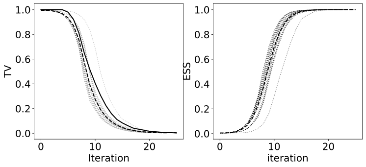
- Conservative compared to SOTA
- Key advantage: No lag/warm-up needed, works from \(t=0\).
Experiment 2: MALA on Stochastic Volatility
A high-dimensional (\(d=2500\)) model.
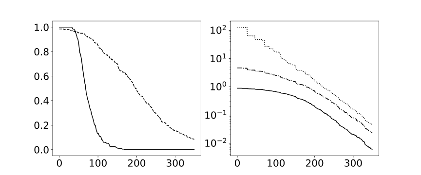
- Still conservative compared to SOTA, but less so than in the previous example: we can benefit from a warm-start.
- Provides bounds for any \(f\)-divergence simultaneously.
Bonus: From Diagnostic to Estimator
The weights \(W_t^n\) used for the \(f\)-divergence bound can instead correct an expectation \(\mathbb{E}[\varphi]\).
Naive time-average: \[\begin{equation} \hat{I}_T^{\text{avg}}(\varphi) = \frac{1}{T}\sum_{t=1}^{T}\sum_{n=1}^{2N} W_t^n \varphi(X_t^n) \end{equation}\]
Square-root rule (Owen and Zhou 2019): \[\begin{equation} \hat{I}_T^{\sqrt{t}}(\varphi) = \frac{\displaystyle\sum_{t=1}^{T} \sqrt{t}\sum_{n=1}^{2N} W_t^n \varphi(X_t^n)}{\displaystyle\sum_{t=1}^{T}\sqrt{t}} \end{equation}\]
Up-weights later iterations, whose weights are more harmonized (lower variance), without having to estimate the variance decay rate.
Experiment 3: Correcting Expectations
Pólya-Gamma logistic regression, \(\varphi(\beta) = \partial_\sigma \log p(\beta;\sigma)\) (sensitivity of the log-prior to its scale), \(N=20\) pairs, 100 repeats.
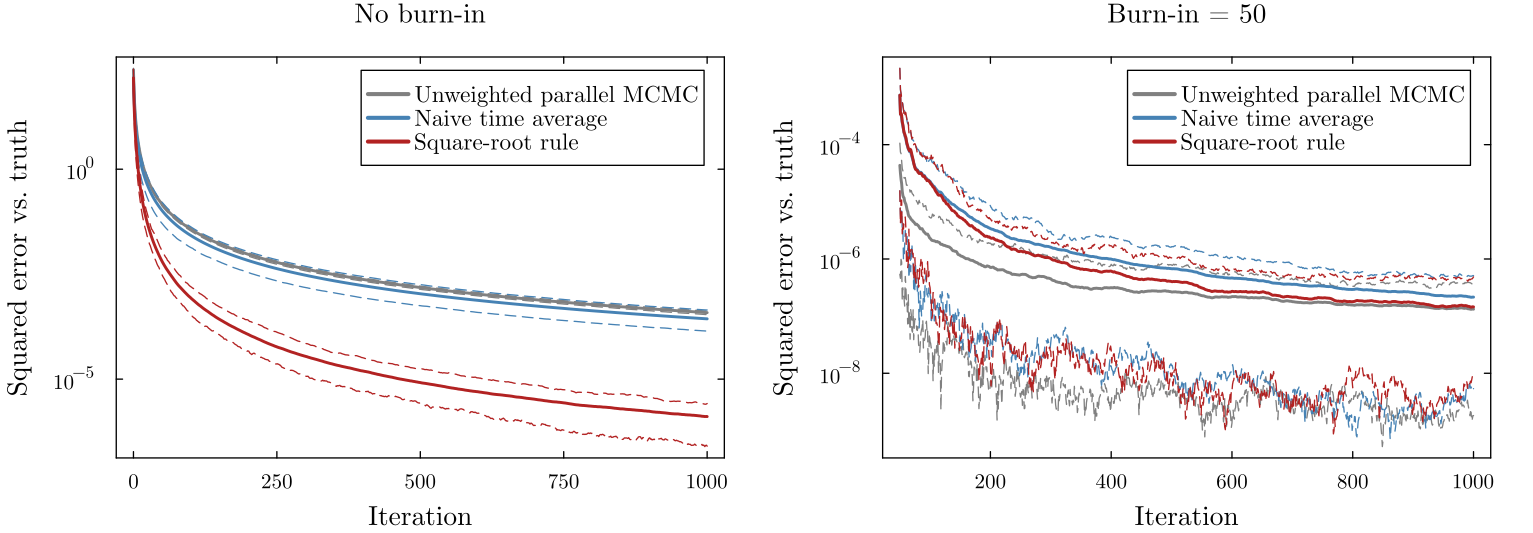
- Without burn-in, the naive average is dragged down by the (degenerate) few weights; the square-root rule is up to 300\(\times\) more accurate.
- A burn-in achieves almost the same effect but you’d need to choose a burn-in length, which is not trivial in practice.
Summary
We introduced a new method for MCMC convergence diagnostics based on weight harmonization.
- It uses couplings to progressively average importance weights between parallel chains.
- This provides consistent, online, non-increasing upper bounds for any \(f\)-divergence.
- The diagnostic is guaranteed to converge to zero for ergodic chains.
- It is easy to implement if a coupled kernel is available.
Limitations and Future Work
The main limitation is the conservativeness of the bound, especially for large \(2N\). This is due to the pairwise interaction scheme.
Potential Improvements:
Rao-Blackwellization: Instead of picking one random pairing, can we average over all possible pairings? This would dramatically increase interaction but is computationally challenging.
Offline Correction: The current method is a “filtering” approach. Can we use ideas from particle smoothing (a “backward pass”) to refine the weights after the run is complete?
Variance Reduction: Incorporate control variates to accelerate the convergence of the diagnostic itself.
Some recent news
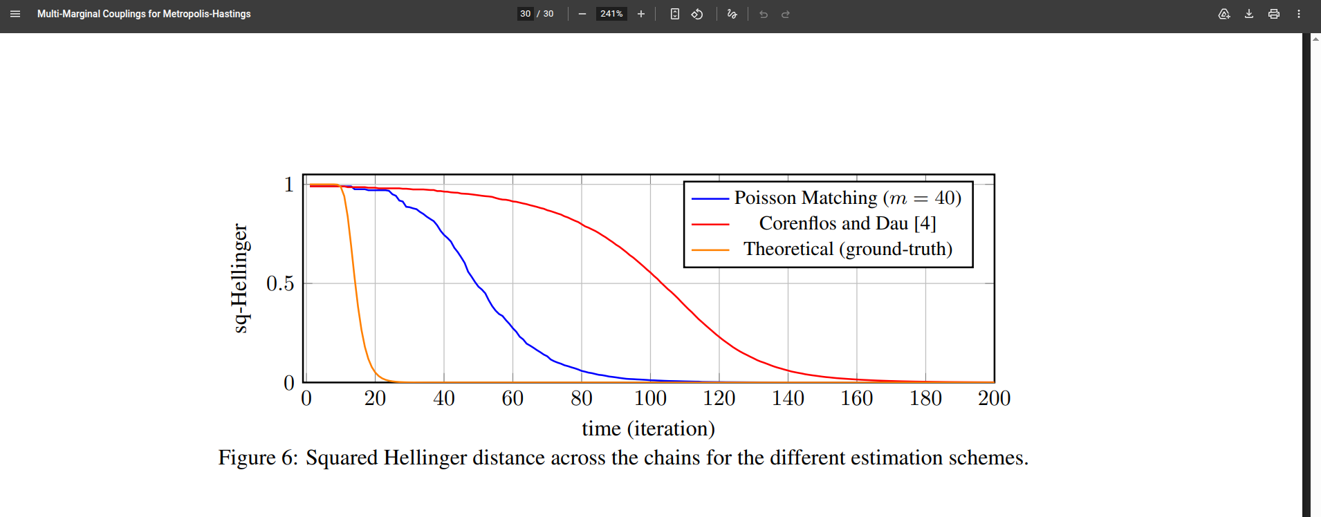
A recent paper just appeared on arXiv: Multi-Marginal Couplings for Metropolis–Hastings by Buu Phan, Gergely Flamich, Ashish Khisti, Shahab Asoodeh, which proposes somthing that kind of can be seen as a Rao–Blackwellized version of our method.
To be continued…
Thank you!
Proof Techniques: Overview
- The theoretical guarantees of our approach rest on several key proofs.
- Consistency ensures the weighted estimates target the correct expectations.
- Decreasing bounds ensures the calculated \(f\)-divergence bound tightens monotonically.
- Ergodic Weight Convergence demonstrates that the variance in the weights decreases exponentially.
- Almost Sure Convergence shows that the weights converge asymptotically to a uniform distribution.
Consistency (Theorem 2)
- We want to show the estimator \(\hat{\theta}_t = \frac{1}{2N} \sum_{n=1}^{2N} w_t^n \varphi(X_t^n)\) is consistent.
- Methodology: Proof proceeds by induction on time \(t\).
- We bound the conditional variance: \(\mathbb{P}\left( \hat\theta_t-\theta_{t-1} \geq \varepsilon \mid \mathcal F_{t-1} \right)\)
- By employing Chebyshev’s inequality and repeatedly applying Jensen’s inequality across the coupling updates, we find: \[ \mathbb{P}\left( \hat\theta_t-\theta_{t-1}\geq \varepsilon \right) \leq \frac{1}{\varepsilon^2N} E[(w_0^1)^2 K^t[\varphi^2](X_0^1)] \]
- Because the RHS is \(\mathcal{O}(1/N)\), the difference vanishes in probability as \(N \to \infty\).
Decreasing Bounds (Proposition 2)
- We must show \(\sum_{n=1}^{2N} f(N W_{t+1}^n) \leq \sum_{n=1}^{2N} f(N W_t^n)\).
- During the update, paired particles \((n, m^n)\) have their weights averaged if they couple: \[ W_{t+1}^n = W_{t+1}^{m^n} = \frac{W_t^n + W_t^{m^n}}{2} \]
- By the convexity of the \(f\)-divergence function \(f\), Jensen’s inequality yields: \[ f(N W_{t+1}^n) + f(N W_{t+1}^{m^n}) \leq f(N W_t^n) + f(N W_t^{m^n}) \]
- Since uncoupled pairs maintain their weights, the entire sum across all pairs is non-increasing.
Ergodic Weight Convergence (Theorem 3)
- We study the squared Euclidean distance to uniform weights: \(V_t = \|W_t - \bar{W}\|_2^2\).
- \(V_t\) acts as a Lyapunov function for the system.
- We utilize the algebraic identity: \[ (x-y)^2 + (x + y - 2z)^2 = 2 [(x-z)^2 + (y-z)^2] \]
- Applied to the pairwise weight averaging \(W_{t+1} = \frac{W_t^n + W_t^{m_t^n}}{2}\), the distance strictly contracts in expectation at every two steps.
- This concludes that the weight variance decreases exponentially fast.
Almost Sure Convergence (Theorem 4)
- Formulates weight harmonization mathematically as an orthogonal projection.
- The averaging \(W_{t+1}^n = W_{t+1}^{m^n}\) is effectively a multiplication by an interaction matrix \(H^{ij}\), where \(H^{ij}_{ii} = H^{ij}_{jj} = H^{ij}_{ij} = 1/2\).
- \(H^{ij}\) projects onto the hyperplane \(L_{ij} = \{x \in \mathbb{R}^{2N} \mid x_i = x_j\}\).
- Relies on novel lemmas for functional analysis: an infinite sequence of orthogonal projections onto a finite set of subspaces converges almost surely to the projection onto their intersection.
- The intersection of all \(L_{ij}\) is perfect uniformity (\(x_1 = x_2 = \dots = x_{2N}\)).