Local geometric convergence of coordinate ascent variational inference
Joint work with Rocco Caprio (Bocconi University) and Sam Power (University of Bristol)
University of Warwick
Mean-field inference and coordinate ascent
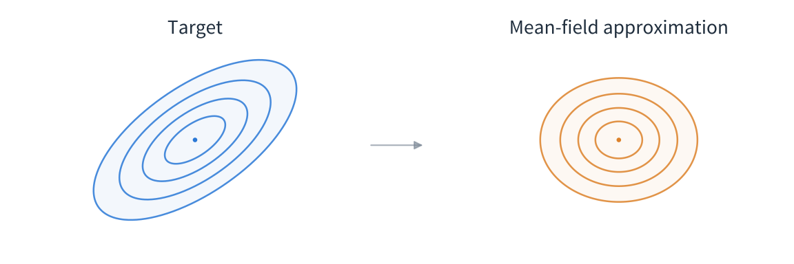
Mean-field inference approximates a joint law by independent blocks
A posterior \pi(x)\propto p(x)p(y\mid x) may be difficult to integrate or sample. Mean-field inference restricts the approximation to a product over M blocks: x=(x_1,\ldots,x_M),\qquad q(x)=\prod_{i=1}^M q_i(x_i).
y: observed data; p(x): prior; p(y\mid x): likelihood; q_i: approximating distribution for block i.
Mean-field inference minimizes Kullback–Leibler divergence
Write \pi=\widetilde\pi/Z, where \widetilde\pi is the unnormalized target and Z=\int\widetilde\pi(x)\,\mathrm dx. Optimize over the factor distributions: \min_{q_1,\ldots,q_M}\operatorname{KL}(q\Vert\pi),\qquad q=\bigotimes_iq_i, \operatorname{KL}(q\Vert\pi)=\int q(x)\log\frac{q(x)}{\pi(x)}\,\mathrm dx.
With factor entropy H(q_i)=-\mathbb E_{q_i}\log q_i, we have \operatorname{KL}(q\Vert\pi)=\log Z-\underbrace{\left\{\mathbb E_q\log\widetilde\pi(X)+\sum_iH(q_i)\right\}}_{\text{evidence lower bound: }\operatorname{ELBO}(q)}.
Minimizing KL is equivalent to maximizing the ELBO.
\bigotimes_iq_i: the joint law with independent factors q_i; M: number of blocks.
Coordinate ascent updates one factor distribution at a time
A coordinate is an entire distribution q_i. With q_{-i}=\bigotimes_{j\ne i}q_j fixed, T_i(q_{-i})=\underset{\nu_i}{\operatorname{argmin}}\; \operatorname{KL}(\nu_i\otimes q_{-i}\Vert\pi) .
The exact coordinate solution is T_i(q_{-i})(x_i)=\frac{\exp\{\mathbb E_{q_{-i}}\log\widetilde\pi(x_i,X_{-i})\}} {\int\exp\{\mathbb E_{q_{-i}}\log\widetilde\pi(u,X_{-i})\}\,\mathrm du}.
Indeed, the objective splits into \operatorname{KL}(\nu_i\otimes q_{-i}\Vert\pi) =\operatorname{KL}(\nu_i\Vert T_i(q_{-i}))+C(q_{-i}), C(q_{-i}) is constant in \nu_i.
Coordinate ascent variational inference (CAVI). Tractable examples include Gaussian targets and conjugate or augmented models.
\nu_i: candidate factor law; q_{-i}=\bigotimes_{j\ne i}q_j; \pi\propto\widetilde\pi: target and unnormalized target density.
Parallel and sequential CAVI use different inputs
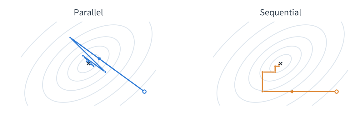
One round updates all M factors, using the same coordinate minimizers T_i.
Parallel
q_i^{k+1}=T_i(q_{-i}^{k}),\qquad i=1,\ldots,M.
Use the old factors for every update.
For three factors, the inputs are \begin{aligned} q_1^{k+1}&=T_1(q_2^k\otimes q_3^k),\\ q_2^{k+1}&=T_2(q_1^k\otimes q_3^k),\\ q_3^{k+1}&=T_3(q_1^k\otimes q_2^k). \end{aligned}
Sequential
q_i^{k+1}=T_i(q_{<i}^{k+1}\otimes q_{>i}^{k}).
Visit i=1,\ldots,M; reuse each new factor immediately.
For three factors, the inputs are \begin{aligned} q_1^{k+1}&=T_1(q_2^k\otimes q_3^k),\\ q_2^{k+1}&=T_2(\textcolor{#2a78d6}{q_1^{k+1}}\otimes q_3^k),\\ q_3^{k+1}&=T_3(\textcolor{#2a78d6}{q_1^{k+1}}\otimes\textcolor{#2a78d6}{q_2^{k+1}}). \end{aligned}
T_i(q_{-i})=\arg\min_{\nu_i}\operatorname{KL}(\nu_i\otimes q_{-i}\Vert\pi), where \pi is the target and q_{-i}=\bigotimes_{j\ne i}q_j.
q_i^k: factor i after k complete rounds; q_{<i}=\bigotimes_{j<i}q_j, q_{>i}=\bigotimes_{j>i}q_j.
Earlier convergence results use correlation or log-concavity
| Work | Setting | Guarantee |
|---|---|---|
| Bhattacharya–Pati–Yang (2025) | Small generalized correlation; two-block algorithms | Global/local geometric contraction in symmetrized KL; global multiblock parallel extension |
| Arnese–Lacker (2026) | Sequential updates; log-concave target with a smooth potential | O(k^{-1}) objective gap; geometric under strong log-concavity |
| Lavenant–Zanella (2024) | Random scan; log-concavity and block smoothness | O(k^{-1}) expected objective gap; geometric under strong log-concavity |
Here the objective gap is \operatorname{KL}(q^k\Vert\pi)-\min_{q\text{ product}}\operatorname{KL}(q\Vert\pi).
Our approach: direct Wasserstein bounds from local sensitivity of the update maps and regularity of the limiting variational factors. The same influence matrix controls parallel, sequential and random-scan updates.
k: complete sweeps for the sequential result, individual coordinate updates for random scan; q^k: current product approximation; \pi: target law.
Gaussian heuristics: CAVI as a linear-system solver
The Gaussian mean-field problem
Let \pi=\mathcal N(\mu,Q^{-1}), with mean \mu and positive-definite precision Q. Use unrestricted scalar factor densities: \min_{q_1,\ldots,q_M}\operatorname{KL}(q\Vert\pi),\qquad q=\bigotimes_iq_i.
Write m_i=\mathbb E_{q_i}X_i and s_i^2=\operatorname{Var}_{q_i}(X_i). Independence gives \begin{aligned} \operatorname{KL}(q\Vert\pi) &=\tfrac12(m-\mu)^\top Q(m-\mu)\\ &\quad+\tfrac12\sum_iQ_{ii}s_i^2-\sum_iH(q_i)+C_\pi, \end{aligned}
At fixed means and variances, the Gaussian maximizes entropy: H(q_i)\leq\tfrac12\log(2\pi e s_i^2), with equality for q_i=\mathcal N(m_i,s_i^2). Thus Gaussian factors attain the minimum.
m=(m_1,\ldots,m_M)^\top: factor means; H(q_i)=-\mathbb E_{q_i}\log q_i: entropy; M: number of factors; C_\pi: constant independent of q.
The remaining optimization is a quadratic in the means
For q_i=\mathcal N(m_i,s_i^2), the objective is exactly \begin{aligned} \operatorname{KL}(q\Vert\pi) &=\tfrac12(m-\mu)^\top Q(m-\mu)\\ &\quad+\tfrac12\left[\sum_i\{Q_{ii}s_i^2-\log s_i^2\}-M-\log\det Q\right]. \end{aligned}
Each variance is calibrated independently of the means: \frac{\partial\operatorname{KL}}{\partial s_i^2} =\tfrac12\left(Q_{ii}-\frac1{s_i^2}\right)=0 \quad\Longrightarrow\quad s_i^2=Q_{ii}^{-1}.
After substituting these variances, \operatorname{KL}(q\Vert\pi) =\tfrac12(m-\mu)^\top Q(m-\mu) +\underbrace{\tfrac12\log\frac{\prod_iQ_{ii}}{\det Q}}_{\operatorname{KL}(q_\star\Vert\pi)}.
The optimum is m=\mu, with q_\star=\bigotimes_i\mathcal N(\mu_i,Q_{ii}^{-1}).
\pi=\mathcal N(\mu,Q^{-1}): target; q=\bigotimes_iq_i; m=(m_i)_{i=1}^M: factor means; s_i^2: factor variances; M: number of factors.
The Gaussian factor distributions evolve under both schedules
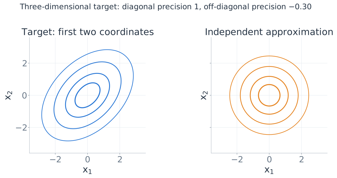
Three-dimensional target: \pi=\mathcal N(0,Q^{-1}), Q_{ii}=1, Q_{ij}=-c (i\ne j, 0\leq c<1/2).
After calibrating the variances, q_i=\mathcal N(m_i,1) and a coordinate update sets m_i\leftarrow c\sum_{j\ne i}m_j.
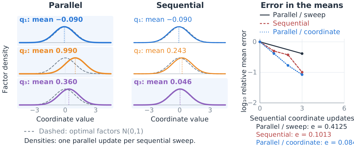
Start: m^0=(2.4,-1.2,0.9); default c=0.30. Error: e(m)=\max_i|m_i|/\max_i|m_i^0|. One clock step is one sequential coordinate update. Parallel curves: one full update per sweep (black) or coordinate (blue).
The Gaussian schedules split the precision matrix differently
Let \delta m^k=m^k-\mu and write Q=D+L+U,\qquad D=\operatorname{diag}(Q_{11},\ldots,Q_{MM}), where L is strictly lower triangular and U=L^\top.
The parallel and sequential mean updates give \begin{aligned} \text{Parallel:}\qquad D\,\delta m^{k+1}&=-(L+U)\,\delta m^k,\\ \text{Sequential:}\qquad(D+L)\,\delta m^{k+1}&=-U\,\delta m^k. \end{aligned}
These are exactly the Jacobi and Gauss–Seidel matrix iterations: \underbrace{B=I-D^{-1}Q}_{\text{Jacobi}},\qquad\underbrace{-(D+L)^{-1}U}_{\text{Gauss--Seidel}}.
Gauss–Seidel converges for every Q\succ0. A complete sequential sweep strictly decreases \tfrac12(m-\mu)^\top Q(m-\mu) unless m=\mu.
\pi=\mathcal N(\mu,Q^{-1}): target; m_i^k=\mathbb E_{q_i^k}X_i: current factor mean; \delta m^k=m^k-\mu: mean error.
The scaled precision determines Jacobi convergence
For target precision Q\succ0, set D=\operatorname{diag}(Q_{11},\ldots,Q_{MM}) and define S=D^{-1/2}QD^{-1/2},\qquad z^k=D^{1/2}(m^k-\mu). The Jacobi mean iteration becomes z^{k+1}=(I-S)z^k. Each eigenvalue \lambda of S multiplies its error mode by 1-\lambda at each round.
Convergence from every initial mean holds exactly when \lambda_{\max}(S)<2\qquad\Longleftrightarrow\qquad 2D-Q\succ0. Positive definiteness gives \lambda>0; convergence also requires \lambda<2.
Under this condition, the worst-case contraction factor is r_Q=\max_j|1-\lambda_j(S)|,\qquad \|m^k-\mu\|_D\leq r_Q^k\|m^0-\mu\|_D,
\pi=\mathcal N(\mu,Q^{-1}): target; m_i^k=\mathbb E_{q_i^k}X_i; \|v\|_D=(v^\top Dv)^{1/2}. \lambda_j(S): eigenvalues of S; \lambda_{\max}(S): largest eigenvalue.
Linearizing a factor update gives its local influence operators
The coordinate minimizer is T_i(q_{-i})=\underset{\nu_i}{\operatorname{argmin}}\, \operatorname{KL}(\nu_i\otimes q_{-i}\Vert\pi),\qquad q_{-i}=\bigotimes_{j\ne i}q_j.
At a fixed point q_i^\star=T_i(q_{-i}^\star), write nearby factors as q_i=q_i^\star(1+h_i),\qquad \mathbb E_{q_i^\star}h_i=0.
Assume the updated relative density is Fréchet differentiable in h at zero. For j\ne i, define A_{ij}h_j=\left.\frac{\mathrm d}{\mathrm dt} \frac{T_i\!\left(q_{-i}^\star(1+t h_j)\right)}{q_i^\star}\right|_{t=0},\qquad A_{ii}=0.
The updated perturbation therefore satisfies h_i^+=\frac{T_i(q_{-i})}{q_i^\star}-1 =\sum_{j\ne i}A_{ij}h_j+o(\|h\|).
\pi: target; \nu_i: candidate factor. q_{-i}^\star(1+t h_j) perturbs only factor j. h=(h_i)_i, \|h\|^2=\sum_i\mathbb E_{q_i^\star}h_i^2; the o(\|h\|) remainder divided by \|h\| tends to zero.
Linearization gives Jacobi and Gauss–Seidel operators
The linear response blocks satisfy h_i^+=\sum_{j\ne i}A_{ij}h_j+o(\|h\|). Set A=(A_{ij})=A_L+A_U, with A_{ii}=0 and strictly lower/upper block parts A_L,A_U.
| Schedule | First-order update near the fixed point |
|---|---|
| Parallel: all inputs old | h^{k+1}=Ah^k+o(\|h^k\|) |
| Sequential: reuse new inputs | h^{k+1}=A_Lh^{k+1}+A_Uh^k+o(\|h^k\|) |
For the linearized fixed-point equations (I-A)h=0, the iteration operators are \underbrace{A}_{\text{block Jacobi}},\qquad \underbrace{(I-A_L)^{-1}A_U}_{\text{block Gauss--Seidel}}.
For Gaussian targets, the corresponding recurrences in the means are exact.
h_i=q_i/q_i^\star-1: relative perturbation; q_i^\star: fixed-point factor; h_i^+: perturbation after updating factor i. \|h\|^2=\sum_i\mathbb E_{q_i^\star}h_i^2; o(\|h\|)/\|h\|\to0 in norm.
From heuristics to the general case: functional inequalities
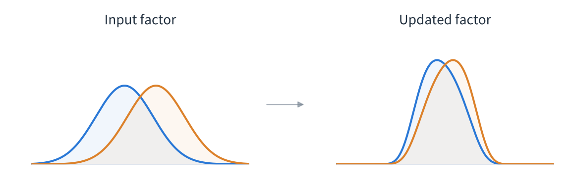
Measuring distance between distributions
For laws with finite second moments, W_2^2(\nu,\gamma)=\inf_{(X,Y):\,X\sim\nu,\,Y\sim\gamma}\mathbb E\|X-Y\|^2.
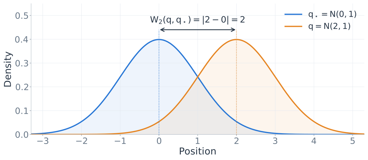
For X\sim\mathcal N(m,\Sigma), take Y=X+(m_\star-m). This coupling attains the lower bound \mathbb E\|X-Y\|^2\geq\|\mathbb EX-\mathbb EY\|^2=\|m-m_\star\|^2.
Hence W_2(\mathcal N(m,\Sigma),\mathcal N(m_\star,\Sigma))=\|m-m_\star\|_2.
\Sigma: common covariance; m,m_\star: current and reference means. W_2: least root mean square displacement over couplings with the prescribed marginals.
Smooth updates and regular limiting factors
The relative Fisher information is \mathcal I(\nu\Vert\gamma)=\int\left\|\nabla\log\frac{\mathrm d\nu}{\mathrm d\gamma}\right\|^2\,\mathrm d\nu.
1. Local smoothness, for all inputs with W_2(q_j,q_j^\star)<\varepsilon_j, j\ne i: \sqrt{\mathcal I(T_i(q_{-i})\Vert q_i^\star)} \leq\sum_{j\ne i}L_{ij}W_2(q_j,q_j^\star).
2. Regularity of the limiting factor, for every admissible \nu: \lambda_i W_2(\nu,q_i^\star)\leq\sqrt{\mathcal I(\nu\Vert q_i^\star)},\qquad\lambda_i>0.
Strong convexity of -\log q_i^\star is sufficient; the condition is more permissive. It concerns the limiting variational factors q_i^\star, not the joint target \pi or its true marginals.
T_i(q_{-i})=\arg\min_{\nu_i}\operatorname{KL}(\nu_i\otimes q_{-i}\Vert\pi); q_{-i}=\bigotimes_{j\ne i}q_j; q_i^\star=T_i(q_{-i}^\star). \pi: target; \varepsilon_j>0: neighbourhood radius; L_{ij}\geq0. W_2: least root mean square displacement over couplings of its two arguments.
The same splitting controls nonlinear Wasserstein errors
Define the factor errors and collect them into a vector: e_i^k=W_2(q_i^k,q_i^\star),\qquad \boldsymbol e^k=(e_1^k,\ldots,e_M^k)^\top. Choose nonnegative coefficients controlling each local factor update: e_i^+\leq\sum_{j\ne i}R_{ij}e_j,\qquad R_{ii}=0. Split R=R_L+R_U into strictly lower and upper triangular parts.
While each coordinate-update input lies in the smoothness neighbourhood, \begin{aligned} \text{Parallel:}\quad&\boldsymbol e^{k+1}\leq R\boldsymbol e^k,\\ \text{Sequential:}\quad&\boldsymbol e^{k+1}\leq (I-R_L)^{-1}R_U\boldsymbol e^k. \end{aligned}
Spectral radius \rho(R)<1 gives local geometric convergence for both schedules.
For a Gaussian target with precision Q, R_{ij}=|Q_{ij}|/Q_{ii} for i\ne j.
q_i^k: factor i after k rounds; q_i^\star: fixed-point factor. e_j=W_2(q_j,q_j^\star): input error; e_i^+: error after updating factor i. W_2: least root mean square coupling displacement. Vector inequalities are componentwise.
One parallel update gives a matrix inequality
For inputs in the smoothness neighbourhood, the parallel update is q_i^{k+1}=\arg\min_{\nu_i}\operatorname{KL}\!\left(\nu_i\otimes\bigotimes_{j\ne i}q_j^k\,\middle\Vert\,\pi\right).
\begin{aligned} \lambda_i e_i^{k+1} &\leq\sqrt{\mathcal I(q_i^{k+1}\Vert q_i^\star)} &&\text{regularity},\\[0.35em] &\leq\sum_{j\ne i}L_{ij}e_j^k &&\text{smoothness, all inputs old}. \end{aligned}
Divide by \lambda_i>0 and set R_{ij}=L_{ij}/\lambda_i for i\ne j, R_{ii}=0. Since L_{ij}\geq0, \boxed{\boldsymbol e^{k+1}\leq R\boldsymbol e^k} \quad\Longrightarrow\quad\boldsymbol e^k\leq R^k\boldsymbol e^0, provided every intermediate iterate stays in the smoothness neighbourhood.
e_i^k=W_2(q_i^k,q_i^\star); \boldsymbol e^k=(e_i^k)_i; q_i^\star: fixed-point factor; \pi: target. Relative Fisher information: \mathcal I(\nu\Vert\gamma)=\int\|\nabla\log(\mathrm d\nu/\mathrm d\gamma)\|^2\,\mathrm d\nu.
Positive weights turn the comparison into contraction
Choose a contraction factor r with \rho(R)<r<1. Positive weights satisfying Rw\leq rw exist: for example, w=(I-R/r)^{-1}\mathbf1=\sum_{\ell=0}^{\infty}(R/r)^\ell\mathbf1, \qquad Rw=r(w-\mathbf1)<rw. Define a weighted maximum error, E_k=\max_i\frac{e_i^k}{w_i},\qquad\text{so that }e_j^k\leq E_kw_j.
Then, for each i, e_i^{k+1}\leq\sum_jR_{ij}e_j^k \leq E_k(Rw)_i\leq rE_kw_i.
Divide by w_i and take the maximum: \boxed{E_{k+1}\leq rE_k.}
e_i^k=W_2(q_i^k,q_i^\star): error to fixed-point factor q_i^\star. R\geq0 is the matrix in e_i^{k+1}\leq\sum_jR_{ij}e_j^k; \rho(R): largest eigenvalue modulus; \mathbf1=(1,\ldots,1)^\top. W_2: least root mean square coupling displacement.
The local neighbourhood remains invariant
Smoothness holds when W_2(q_i,q_i^\star)<\varepsilon_i. Start sufficiently close that E_0<\min_i\frac{\varepsilon_i}{w_i}.
If E_k\leq E_0, then e_i^k\leq w_iE_k\leq w_iE_0<\varepsilon_i. Therefore E_{k+1}\leq rE_k\leq E_0.
Induction gives the explicit factorwise bound \boxed{\max_i\frac{W_2(q_i^k,q_i^\star)}{w_i} \leq r^k\max_i\frac{W_2(q_i^0,q_i^\star)}{w_i}.}
A product coupling gives W_2(\bigotimes_iq_i^k,\bigotimes_iq_i^\star)\leq\|w\|_2\,r^kE_0 in the Euclidean product metric.
q_i^\star: fixed-point factor; e_i^k=W_2(q_i^k,q_i^\star); E_k=\max_i e_i^k/w_i. The fixed weights w_i>0 give E_{k+1}\leq rE_k, 0<r<1, whenever every factor error is below its radius \varepsilon_i.
Applications: logistic regression and Gaussian mixtures
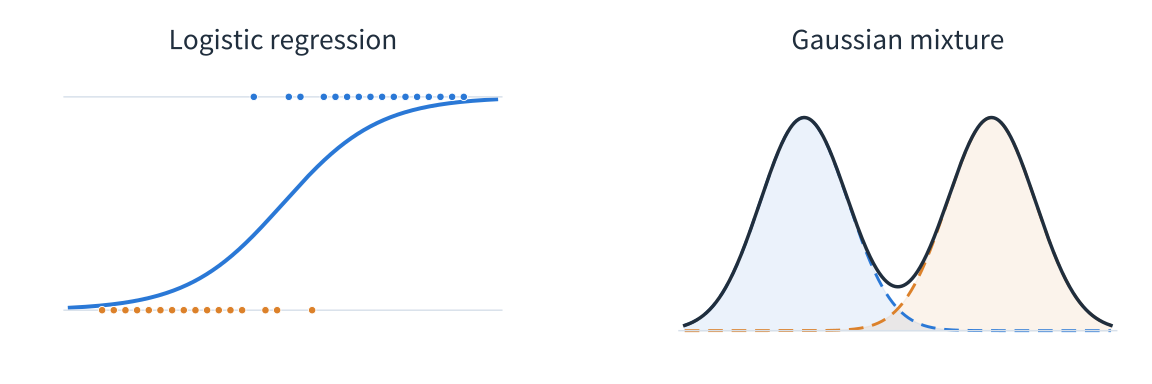
Auxiliary variables give a composed update
Let \beta be the model parameter and z the auxiliary variables. Approximate their posterior by q_\beta\otimes q_z. One sequential sweep defines \mathcal T:
\begin{aligned} q_z^{k+1}&=\underset{\nu_z}{\operatorname{argmin}}\, \operatorname{KL}(q_\beta^k\otimes\nu_z\Vert\pi),\\[0.25em] q_\beta^{k+1}&=\underset{\nu_\beta}{\operatorname{argmin}}\, \operatorname{KL}(\nu_\beta\otimes q_z^{k+1}\Vert\pi) =\mathcal T(q_\beta^k). \end{aligned}
At a fixed point q_\beta^\star=\mathcal T(q_\beta^\star), set e_k=W_2(q_\beta^k,q_\beta^\star). The local comparison is \lambda e_{k+1}\leq \sqrt{\mathcal I\!\left(\mathcal T(q_\beta^k)\Vert q_\beta^\star\right)} \leq L e_k.
Here \lambda>0 controls regularity of the limiting parameter factor, and L\geq0 controls sensitivity of the complete sweep. If L/\lambda<1, the parameter error contracts locally.
\pi: augmented posterior; \nu_z,\nu_\beta: candidate factor laws. \mathcal I(\nu\Vert\gamma)=\int\|\nabla\log(\mathrm d\nu/\mathrm d\gamma)\|^2\,\mathrm d\nu. W_2: least root mean square coupling displacement.
Bayesian logistic regression
For binary observations y_i and covariates x_i\in\mathbb R^p, i=1,\ldots,n, use coefficients \beta\in\mathbb R^p: \Pr(Y_i=1\mid\beta)=\sigma(x_i^\top\beta),\qquad \beta\sim\mathcal N(m_{\mathrm{pr}},Q_0^{-1}),\qquad Q_0\succ0, where \sigma(t)=(1+e^{-t})^{-1}.
Introduce Pólya–Gamma variables \omega_i. The augmented posterior log density is
\begin{aligned} \log\pi(\beta,\omega) &=-\tfrac12\beta^\top\!\left[Q_0+X^\top\operatorname{diag}(\omega)X\right]\beta\\ &\quad+\beta^\top\!\left[X^\top(y-\tfrac12\mathbf1)+Q_0m_{\mathrm{pr}}\right]+C(\omega). \end{aligned}
We fit q_\beta\otimes\prod_iq_{\omega_i}. Averaging over the auxiliary factors leaves a quadratic in \beta, so the exact parameter update is Gaussian.
X: design matrix with rows x_i^\top; y=(y_1,\ldots,y_n)^\top; \mathbf1: all-ones vector. m_{\mathrm{pr}},Q_0: prior mean and precision; C(\omega) is constant in \beta.
Pólya–Gamma weights give a Gaussian update
Starting from q_\beta^k=\mathcal N(m_k,\Sigma_k), define c_{i,k}\geq0 using the second moment c_{i,k}^2=\mathbb E_{q_\beta^k}[(x_i^\top\beta)^2] =(x_i^\top m_k)^2+x_i^\top \Sigma_kx_i.
q_{\omega_i}^{k+1}=\operatorname{PG}(1,c_{i,k}),\qquad w_{i,k+1}=\mathbb E_{q_{\omega_i}^{k+1}}[\omega_i]=\frac{\tanh(c_{i,k}/2)}{2c_{i,k}}.
Averaging the quadratic then gives \begin{aligned} Q_{k+1}&=Q_0+X^\top\operatorname{diag}(w_{k+1})X,\\ q_\beta^{k+1}&=\mathcal N\!\left(Q_{k+1}^{-1}\left[X^\top(y-\tfrac12\mathbf1)+Q_0m_{\mathrm{pr}}\right],Q_{k+1}^{-1}\right). \end{aligned}
X: design matrix with rows x_i^\top; y=(y_i)_{i=1}^n, y_i\in\{0,1\}; \mathbf1: all-ones vector. Prior: \beta\sim\mathcal N(m_{\mathrm{pr}},Q_0^{-1}). \operatorname{PG}: Pólya–Gamma law; w_{k+1}=(w_{i,k+1})_{i=1}^n. At c_{i,k}=0, set w_{i,k+1}=1/4.
Local rates can remain controlled as dimension grows
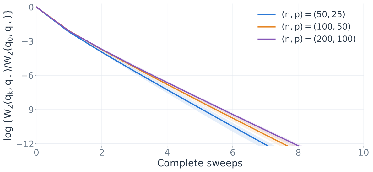
Local experiment. Q_0=X^\top X/8+I_p; 10 datasets per size.
Around each numerical fixed point (m_\star,\Sigma_\star), start with m_0=m_\star+0.1u,\quad \Sigma_0=1.1\Sigma_\star, where \|u\|=1.
Lines: median log relative W_2 error. Shading: interquartile range. The distance includes covariance error.
Let r_\star be the limiting local contraction bound as the neighbourhood shrinks. For prior precision Q_0=X^\top X/g+cI_p, with g,c>0, r_\star^2\leq\frac{1}{1+4/g}<1. \qquad \text{Here }g=8:\quad r_\star\leq\sqrt{2/3}\approx0.817.
X\in\mathbb R^{n\times p}: design for n observations and p coefficients; Q_0: prior precision. q_k=\mathcal N(m_k,\Sigma_k); q_\star=\mathcal N(m_\star,\Sigma_\star): fixed-point factor.
W_2^2(\nu,\gamma)=\inf_{U\sim\nu,\,V\sim\gamma}\mathbb E\|U-V\|_2^2. The plot uses Euclidean distance; the theorem uses \|\Sigma_\star^{-1/2}v\|_2.
A Gaussian mixture can have several variational fixed points
For observations y_1,\ldots,y_n\in\mathbb R^d, use opposite unknown component means \pm\beta: Y_i\sim\alpha\,\mathcal N(\beta,\tau^{-1}I_d) +(1-\alpha)\,\mathcal N(-\beta,\tau^{-1}I_d), \beta\sim\mathcal N(0,\tau_0^{-1}I_d).
The weight \alpha and precisions \tau,\tau_0 are known. Introduce Z_i\sim\operatorname{Bernoulli}(\alpha) with Y_i\mid Z_i,\beta\sim\mathcal N((2Z_i-1)\beta,\tau^{-1}I_d),\qquad q=q_\beta\otimes\prod_iq_{Z_i}.
For the balanced case \alpha=1/2, the coefficient log posterior is \log\pi(\beta\mid y)=-\frac{\tau_0+n\tau}{2}\|\beta\|^2 +\sum_i\log\cosh(\tau y_i^\top\beta)+C. It is unchanged by \beta\mapsto-\beta.
\alpha: weight of the +\beta component; \tau,\tau_0: observation and prior precisions; I_d: identity matrix; C: constant independent of \beta.
Responsibilities and the Gaussian mean take turns
Let m_k=\mathbb E_{q_\beta^k}[\beta]. The allocation probabilities depend only on this mean because \mathbb E_{q_\beta^k}\!\left[\|y_i+\beta\|^2-\|y_i-\beta\|^2\right]=4y_i^\top m_k.
\begin{aligned} q_{Z_i}^{k+1}&=\operatorname{Bernoulli}(r_{i,k+1}),\\ \log\frac{r_{i,k+1}}{1-r_{i,k+1}}&=\log\frac{\alpha}{1-\alpha}+2\tau y_i^\top m_k,\\[0.3em] m_{k+1}&=\frac{\tau}{\tau_0+n\tau}\sum_i(2r_{i,k+1}-1)y_i,\\ q_\beta^{k+1}&=\mathcal N\!\left(m_{k+1},(\tau_0+n\tau)^{-1}I_d\right). \end{aligned}
The covariance is fixed after one sweep. Thus, for k\geq1, W_2(q_\beta^k,q_\beta^\star)=\|m_k-m_\star\|_2.
y_i\in\mathbb R^d: observations, i=1,\ldots,n; \alpha=\Pr(Z_i=1): weight of the +\beta component; observation covariance \tau^{-1}I_d; prior \beta\sim\mathcal N(0,\tau_0^{-1}I_d).
r_{i,k+1}=q_{Z_i}^{k+1}(Z_i=1); q_\beta^\star=\mathcal N(m_\star,(\tau_0+n\tau)^{-1}I_d): selected fixed-point factor.
Different starts can converge to different fixed points
Use 20 scalar observations, balanced weights and unit observation/prior precisions: m_{k+1}=T(m_k),\qquad T(m)=\frac1{21}\sum_{i=1}^{20}y_i\tanh(y_im).
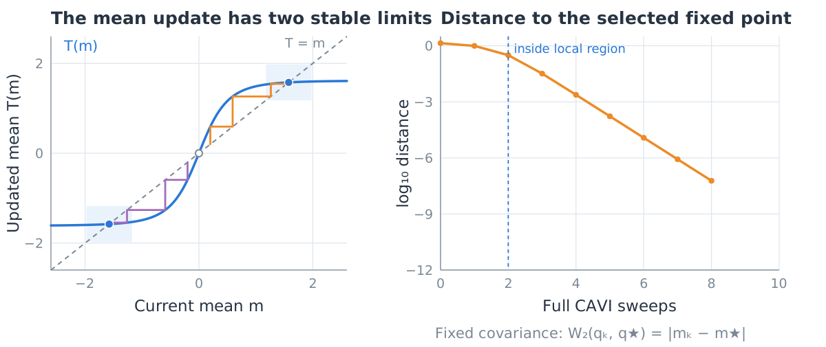
The derivative is T'(m)=\frac1{21}\sum_{i=1}^{20}y_i^2[1-\tanh^2(y_im)].
T'(0)\approx3.15>1: the centre repels. T'(\pm1.577)\approx0.071<1: both nonzero fixed points attract locally.
y_i: observations; m_\star=T(m_\star): selected fixed-point mean. Plot: q_k=\mathcal N(m_k,1/21), q_\star=\mathcal N(m_\star,1/21).
Local geometric convergence appears in the error curves
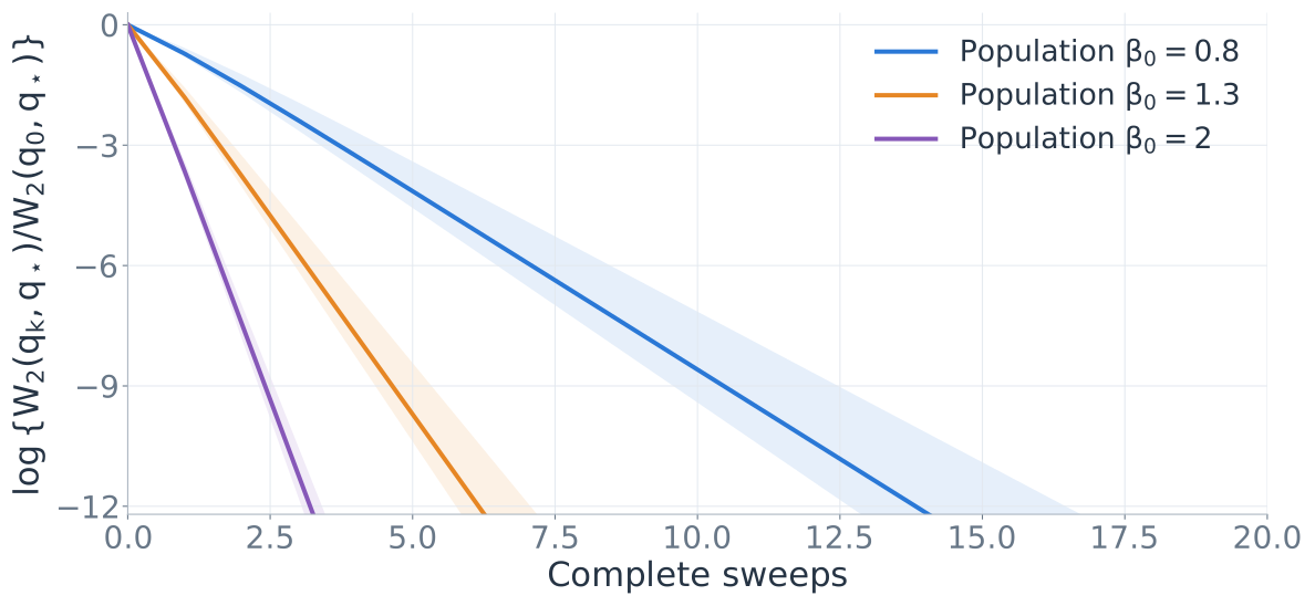
Local experiment. 300 scalar observations; balanced weights; unit observation and prior precisions.
Generating means: \pm\beta_0; their separation is 2\beta_0.
Each run starts at m_0=m_\star-0.15 with covariance 1/301.
Lines: median log relative mean error over 10 datasets per separation. Bands: interquartile range. Each error uses that run’s fixed point.
If r_\varepsilon=\sup_{|m-m_\star|\leq\varepsilon}|T'(m)|<1, then |m_k-m_\star|\leq r_\varepsilon^k|m_0-m_\star|\quad \text{for }|m_0-m_\star|\leq\varepsilon.
The first-order multiplier is T'(m_\star); r_\varepsilon bounds the derivative throughout the neighbourhood.
m_{k+1}=T(m_k), T(m)=\frac1{301}\sum_{i=1}^{300}y_i\tanh(y_im); m_\star=T(m_\star): selected fixed-point mean; \varepsilon: neighbourhood radius.
Plot: q_k=\mathcal N(m_k,1/301), q_\star=\mathcal N(m_\star,1/301) and W_2(q_k,q_\star)=|m_k-m_\star|.
Update sensitivity gives a quantitative convergence proof
For parallel CAVI, the error of each updated factor is controlled by the old factor errors: e_i^k=W_2(q_i^k,q_i^\star),\qquad \boldsymbol e^k=(e_1^k,\ldots,e_M^k)^\top, \qquad\boldsymbol e^{k+1}\leq R\boldsymbol e^k.
If \rho(R)<1, choose positive weights with Rw\leq rw, r<1. Then \max_i\frac{e_i^k}{w_i}\leq r^k\max_i\frac{e_i^0}{w_i} inside a sufficiently small invariant neighbourhood of the variational fixed point.
- First-order structure: Gaussian means follow Jacobi/Gauss–Seidel matrix iterations; differentiable factor updates have the same linearization.
- Nonlinear guarantee: R bounds Wasserstein errors on a neighbourhood, using regularity of the limiting variational factors.
- Augmented models: the same argument controls a complete parameter-to-parameter sweep, as in logistic regression and mixtures.
q_i^k: factor i after k parallel rounds; q_i^\star: fixed-point factor. R\geq0: matrix in the displayed error bound; \rho(R): largest eigenvalue modulus; w_i>0: error weights; r<1: contraction factor. W_2: least root mean square coupling displacement.
What more is in the paper
| Setting | Additional results |
|---|---|
| Random scans | Expected-error bounds when one factor is chosen uniformly at random at each step. |
| Discrete factors | Global geometric convergence in total variation for Ising and Curie–Weiss models under a weak-interaction condition. |
| Probit regression | Global geometric convergence. Under specified prior and design scalings, the rate remains bounded away from one as dimension increases. |
| Non-convex potentials | Global geometric convergence for sufficiently weakly coupled Ginzburg–Landau models with double-well site potentials. |
Discussion
Convergence to a variational fixed point controls computational error. The product approximation can still be inaccurate.
How should we choose blocks and parametrizations to weaken dependence while keeping factor updates tractable?
Can sharper influence criteria from Gibbs sampling extend the convergence guarantees for CAVI?
How much numerical error can we allow when factor updates are computed approximately?
Questions and technical details
Functional inequalities
TI definition · Strong convexity and LSI · TI hierarchy · Non-log-concavity · Lyapunov criterion · TI without LSI · Why LSI fails · Coupled CAVI without LSI · Converse · Tensorization · Geometry · Langevin route
Algorithms, assumptions and guarantees
KL descent · Local assumptions · Checking smoothness · Sequential proof · Random scan · Parallel instability · Conservative bounds · Derivative · Blocking · Error meanings · Stopping and inexact updates · Coordinate descent
Discrete spaces
Discrete TI · Mixed differences · Ising · Curie–Weiss · Comparison with Gibbs
Application calculations
Probit · Prior scaling · Logistic Fisher identity · Finite neighbourhood · Local logistic rate · Multivariate mixtures · Double wells · Spatial Poisson · Data augmentation
Return to discussion. In the HTML presentation, press Q to return here.
TI controls distance by relative Fisher information
For a reference density \gamma on \mathbb R^d, define \mathcal I(\rho\Vert\gamma) =\int\left\|\nabla\log\frac{\rho}{\gamma}(x)\right\|_2^2\rho(x)\,\mathrm dx.
A transportation-information inequality (TI) with constant \lambda>0 is \lambda W_p(\rho,\gamma)\leq\sqrt{\mathcal I(\rho\Vert\gamma)} \qquad\text{for every admissible }\rho.
Here p=1 or 2, with W_p(\rho,\gamma) =\inf_{(X,Y):\,X\sim\rho,\,Y\sim\gamma} \bigl(\mathbb E\|X-Y\|_2^p\bigr)^{1/p}.
W_2–TI implies W_1–TI because W_1\leq W_2; the reverse implication is not automatic.
\rho,\gamma: probability densities; \rho\ll\gamma means absolute continuity. Set \mathcal I=+\infty when the density ratio has no admissible weak gradient. Larger \lambda gives a stronger bound.
Strong convexity and LSI are sufficient for TI
Let \gamma(x)\propto e^{-V(x)} on \mathbb R^d, with V\in C^2 and \lambda>0.
\nabla^2V\succeq\lambda I_d \quad\Longrightarrow\quad \underbrace{\operatorname{KL}(\rho\Vert\gamma) \leq\frac{\mathcal I(\rho\Vert\gamma)}{2\lambda}}_{\text{logarithmic Sobolev inequality (LSI)}}.
LSI also gives the transport-entropy bound W_2^2(\rho,\gamma)\leq\frac{2}{\lambda}\operatorname{KL}(\rho\Vert\gamma).
Combining the two inequalities gives W_2^2(\rho,\gamma)\leq\frac{\mathcal I(\rho\Vert\gamma)}{\lambda^2}.
On a complete Riemannian manifold, replace \nabla^2V by \nabla^2V+\operatorname{Ric}, the potential Hessian plus Ricci curvature.
I_d: identity matrix; \operatorname{KL}(\rho\Vert\gamma)=\int\rho\log(\rho/\gamma); \mathcal I(\rho\Vert\gamma)=\int|\nabla\log(\rho/\gamma)|^2\,\mathrm d\rho; W_2: least root mean square coupling displacement.
TI implies transport-entropy and Poincaré inequalities
Suppose \gamma satisfies \lambda W_2(\rho,\gamma)\leq\sqrt{\mathcal I(\rho\Vert\gamma)} for every admissible \rho, with \lambda>0.
Transport-entropy: W_2^2(\rho,\gamma)\leq\frac{2}{\lambda}\operatorname{KL}(\rho\Vert\gamma). Poincaré: for every admissible test function f, \operatorname{Var}_\gamma(f)\leq\frac1\lambda\int\|\nabla f\|_2^2\,\mathrm d\gamma.
Poincaré alone is insufficient: the Laplace density \gamma(x)=\tfrac12e^{-|x|} satisfies Poincaré but fails W_2–TI.
\operatorname{Var}_\gamma(f)=\int(f-\int f\,\mathrm d\gamma)^2\,\mathrm d\gamma; \nabla f: gradient of f; \operatorname{KL}=\int\rho\log(\rho/\gamma); \mathcal I=\int|\nabla\log(\rho/\gamma)|^2\,\mathrm d\rho; W_2: least root mean square coupling displacement.
A non-log-concave density can still satisfy LSI and TI
Suppose \gamma_0\propto e^{-V_0} satisfies LSI with constant \lambda_0>0. For a bounded perturbation B, \gamma\propto e^{-(V_0+B)},\qquad \operatorname{osc}(B)=\sup B-\inf B, the Holley–Stroock principle gives LSI, and hence W_2–TI, with \lambda\geq\lambda_0e^{-\operatorname{osc}(B)}.
For example, \gamma(x)\propto\exp\!\left(-\frac{x^2}{2}-2\cos x\right),\qquad V''(x)=1-2\cos x. Since V''(0)=-1, this density is not log-concave. Nevertheless, \lambda=e^{-4} is a valid LSI and TI constant.
LSI: \operatorname{KL}(\rho\Vert\gamma)\leq\mathcal I(\rho\Vert\gamma)/(2\lambda); TI: W_2(\rho,\gamma)\leq\sqrt{\mathcal I(\rho\Vert\gamma)}/\lambda; \mathcal I=\int|\nabla\log(\rho/\gamma)|^2\,\mathrm d\rho.
A Lyapunov drift condition gives TI without a curvature bound
For \gamma\propto e^{-V} on \mathbb R^d, define the Langevin generator \mathcal L f=\Delta f-\nabla V\cdot\nabla f.
If a positive function U satisfies \frac{\mathcal L U(x)}{U(x)}\leq b-c\|x-x_0\|_2^2, \qquad b,c>0, then \gamma satisfies W_2–TI with some positive constant.
A useful trial function is U(x)=e^{a\|x\|_2^2}, a>0: \frac{\mathcal L U}{U} =2ad+4a^2\|x\|_2^2-2a\,x\cdot\nabla V(x). An inward drift x\cdot\nabla V(x)\geq\eta\|x\|_2^2-C, with \eta>2a, verifies the condition.
U: Lyapunov test function, with U^{-1} locally bounded; x_0: reference point; d: dimension; a,\eta,c>0, b,C<\infty. W_2–TI means W_2\leq\lambda^{-1}(\int|\nabla\log(\rho/\gamma)|^2\,\mathrm d\rho)^{1/2} for some \lambda>0.
An explicit density satisfies Wasserstein-2 TI but no LSI
On \mathbb R, take \gamma(x)=Z^{-1}e^{-V(x)},\qquad V(x)=|x|^3+3x^2\sin^2x+|x|^{9/4}. For x>0, V'(x)=3x^2(1+\sin2x)+6x\sin^2x+\frac94x^{5/4}, so symmetry gives xV'(x)\geq\frac94|x|^{9/4} on the whole line.
With U(x)=e^{ax^2} and \mathcal L f=f''-V'f', a>0, \frac{\mathcal L U}{U} \leq2a+4a^2x^2-\frac{9a}{2}|x|^{9/4} \leq b-cx^2 for suitable b,c>0. Liu’s criterion therefore gives W_2–TI.
The same density fails every logarithmic Sobolev inequality (LSI); the tail calculation follows.
Z=\int_{\mathbb R}e^{-V(x)}\,\mathrm dx; U: positive test function. W_2–TI: W_2(\rho,\gamma)\leq\lambda^{-1}\sqrt{\mathcal I(\rho\Vert\gamma)} for some \lambda>0, where \mathcal I=\int|\partial_x\log(\rho/\gamma)|^2\,\mathrm d\rho.
The oscillating potential fails the one-dimensional LSI criterion
For \gamma(x)\propto e^{-V(x)} with V(x)=|x|^3+3x^2\sin^2x+|x|^{9/4}, we have V'(x)\to\infty and V''(x)/V'(x)^2\to0 as x\to+\infty.
Under these tail conditions, LSI requires \limsup_{x\to+\infty}\frac{V(x)}{V'(x)^2}<\infty.
At x_k=3\pi/4+k\pi, k=0,1,\ldots, we have \sin(2x_k)=-1 and V'(x_k)=3x_k+\frac94x_k^{5/4},\qquad \frac{V(x_k)}{V'(x_k)^2}\sim\frac{16}{81}\sqrt{x_k}\longrightarrow\infty. Thus no finite logarithmic Sobolev constant exists.
LSI would mean \operatorname{KL}(\rho\Vert\gamma)\leq C\mathcal I(\rho\Vert\gamma) for a finite C, for all admissible \rho; \mathcal I=\int|\partial_x\log(\rho/\gamma)|^2\,\mathrm d\rho. a_k\sim b_k means a_k/b_k\to1.
TI without LSI can yield convergence for a coupled CAVI model
Let V(x)=|x|^3+3x^2\sin^2x+|x|^{9/4} and \gamma(x)=Z^{-1}e^{-V(x)}. This even density satisfies W_2–TI with some \lambda>0, but no LSI.
Couple two such variables through \pi_J(x_1,x_2)\propto e^{-V(x_1)-V(x_2)-Jx_1x_2}. For i\ne j, the exact factor update is T_i(q_j)(x)=\frac{\gamma(x)e^{-Jm_jx}}{\int\gamma(z)e^{-Jm_jz}\,\mathrm dz}, \qquad m_j=\int xq_j(x)\,\mathrm dx.
Since \mathbb E_\gamma X=0, \sqrt{\mathcal I(T_i(q_j)\Vert\gamma)}=|Jm_j| \leq |J|W_2(q_j,\gamma). Thus, if 0<|J|<\lambda, parallel CAVI contracts globally to \gamma\otimes\gamma with factor at most |J|/\lambda per round.
J: interaction strength; Z=\int e^{-V}; q_j: current factor. TI: W_2(\rho,\gamma)\leq\sqrt{\mathcal I(\rho\Vert\gamma)}/\lambda; \mathcal I=\int|\partial_x\log(\rho/\gamma)|^2\,\mathrm d\rho. Initially, \int Vq_j<\infty and \int q_j\log q_j\in\mathbb R.
With curvature bounded below, Wasserstein-2 TI implies LSI
Let \gamma\propto e^{-V}, suppose \nabla^2V\succeq-KI_d for some finite K\geq0, and assume W_2(\rho,\gamma)\leq\lambda^{-1}\sqrt{\mathcal I(\rho\Vert\gamma)}.
The entropy–transport–information inequality gives \operatorname{KL}(\rho\Vert\gamma) \leq W_2(\rho,\gamma)\sqrt{\mathcal I(\rho\Vert\gamma)} +\frac K2W_2^2(\rho,\gamma).
Substitution yields a logarithmic Sobolev inequality (LSI): \operatorname{KL}(\rho\Vert\gamma) \leq\left(\frac1\lambda+\frac{K}{2\lambda^2}\right)\mathcal I(\rho\Vert\gamma).
Therefore a smooth W_2–TI but no LSI example must escape every finite lower bound on curvature.
K: bound on negative curvature; I_d: identity matrix; \operatorname{KL}=\int\rho\log(\rho/\gamma); \mathcal I=\int|\nabla\log(\rho/\gamma)|^2\,\mathrm d\rho; W_2: least root mean square coupling displacement.
Tensorization preserves the weakest factor constant
Suppose each \gamma_j on \mathbb R^{d_j} satisfies W_2(\rho_j,\gamma_j)\leq\lambda_j^{-1}\sqrt{\mathcal I(\rho_j\Vert\gamma_j)},\qquad\lambda_j>0. Equip the product space with squared distance \sum_j\|x_j-y_j\|_2^2 and let \gamma=\bigotimes_{j=1}^J\gamma_j.
For every admissible joint law \rho, W_2^2(\rho,\gamma) \leq\sum_{j=1}^J\frac1{\lambda_j^2} \int\left\|\nabla_j\log\frac{\rho}{\gamma}\right\|_2^2\,\mathrm d\rho \leq\frac{\mathcal I(\rho\Vert\gamma)}{(\min_j\lambda_j)^2}.
The comparison law \rho need not be a product. Increasing the number of independent factors does not itself worsen the TI constant.
J: number of product components; \nabla_j: gradient in component j; \mathcal I(\rho\Vert\gamma)=\sum_j\int\|\nabla_j\log(\rho/\gamma)\|_2^2\,\mathrm d\rho. W_2 uses the displayed product distance.
A weighted distance requires the dual Fisher norm
For a symmetric positive-definite matrix B, use W_{2,B}^2(\rho,\gamma) =\inf_{X\sim\rho,\,Y\sim\gamma}\mathbb E[(X-Y)^\top B(X-Y)]. The matching Fisher information is \mathcal I_B(\rho\Vert\gamma) =\int\left(\nabla\log\frac{\rho}{\gamma}\right)^\top B^{-1}\nabla\log\frac{\rho}{\gamma}\,\mathrm d\rho.
If \gamma\propto e^{-V} and \nabla^2V\succeq B, then W_{2,B}(\rho,\gamma)\leq\sqrt{\mathcal I_B(\rho\Vert\gamma)}. In particular, \gamma=\mathcal N(m,B^{-1}) has constant one in this geometry.
B: metric matrix; B^{-1} weights the gradient because gradients transform in the dual coordinates. m: Gaussian mean. Euclidean error satisfies W_2\leq W_{2,B}/\sqrt{\lambda_{\min}(B)}, where \lambda_{\min}(B) is the smallest eigenvalue.
Langevin contraction supplies a Wasserstein-1 TI bound
Let P_t(x,\cdot) be the time-t law of Langevin diffusion with invariant density \gamma\propto e^{-V} and generator \mathcal L=\Delta-\nabla V\cdot\nabla. Suppose W_1(P_t(x,\cdot),P_t(y,\cdot))\leq\ell(t)\|x-y\|_2, \qquad C=\int_0^\infty\ell(t)\,\mathrm dt<\infty.
For a function f with Lipschitz constant at most one, the centred Poisson solution satisfies -\mathcal L u=f-\mathbb E_\gamma f,\qquad\|\nabla u\|_\infty\leq C.
Integration by parts and transport duality give W_1(\rho,\gamma)\leq C\sqrt{\mathcal I(\rho\Vert\gamma)}. This argument establishes W_1–TI, with \lambda=1/C.
P_t: Langevin transition kernel; \ell(t): contraction bound; C: its time integral; \mathcal I=\int|\nabla\log(\rho/\gamma)|^2\,\mathrm d\rho. W_1: least expected coupling displacement. Lipschitz constant at most one means |f(x)-f(y)|\leq\|x-y\|_2.
One coordinate update decreases KL exactly
For a target density \pi, hold q_{-i}=\bigotimes_{j\ne i}q_j fixed and define T_i(q_{-i})(x_i)=\frac{\exp\{\mathbb E_{q_{-i}}\log\pi(x_i,X_{-i})\}}{Z_i(q_{-i})}, where Z_i(q_{-i}) normalizes the density. Whenever the terms are finite, \operatorname{KL}(q_i\otimes q_{-i}\Vert\pi) =\operatorname{KL}(q_i\Vert T_i(q_{-i}))+C(q_{-i}).
Replacing q_i by T_i(q_{-i}) decreases the joint KL by exactly \operatorname{KL}(q_i\Vert T_i(q_{-i}))\geq0.
Sequential and random-scan updates therefore decrease KL. Simultaneous updates need not do so: each factor was optimized with the other factors held at their old values.
\operatorname{KL}(q\Vert\pi)=\int\log(q/\pi)\,\mathrm dq; C(q_{-i}) does not depend on q_i. Minimizing KL is maximizing the evidence lower bound, up to the fixed log evidence.
Local smoothness and regularity of a fixed-point factor
At a product fixed point q^\star=\bigotimes_iq_i^\star, define the coordinate update by T_i(q_{-i})=\underset{\nu_i}{\operatorname{argmin}}\, \operatorname{KL}(\nu_i\otimes q_{-i}\Vert\pi),\qquad q_i^\star=T_i(q_{-i}^\star).
Smoothness is local in the input laws: for W_p(q_j,q_j^\star)<\varepsilon_j, \sqrt{\mathcal I(T_i(q_{-i})\Vert q_i^\star)} \leq\sum_{j\ne i}L_{ij}W_p(q_j,q_j^\star).
TI is an inequality for the reference law q_i^\star: \lambda_i W_p(\nu_i,q_i^\star)\leq\sqrt{\mathcal I(\nu_i\Vert q_i^\star)} \quad\text{for every admissible }\nu_i.
Only the reference factor must satisfy TI. It is a variational factor, generally different from a true posterior marginal or a full conditional.
q_{-i}=\bigotimes_{j\ne i}q_j; W_p(\mu,\nu)=\inf_{X\sim\mu,Y\sim\nu}(\mathbb E\|X-Y\|^p)^{1/p}; \mathcal I(\mu\Vert\nu)=\int\|\nabla\log(\mathrm d\mu/\mathrm d\nu)\|^2\,\mathrm d\mu. L_{ij}\geq0, \lambda_i,\varepsilon_i>0.
Mixed derivatives give checkable smoothness constants
For \pi(x)\propto e^{-f(x)} on Euclidean blocks, suppose \sup_x\|\nabla^2_{x_i x_j}f(x)\|_{\mathrm{op}}\leq L_{ij},\qquad i\ne j. The normalized coordinate density satisfies T_i(q_{-i})(x_i)\propto e^{-\mathbb E_{q_{-i}}f(x_i,X_{-i})},\qquad \nabla\log T_i(q_{-i})=-\mathbb E_{q_{-i}}\nabla_i f.
Couple each pair of input factors, then use the mixed-derivative bounds: \left\|\nabla\log\frac{T_i(q_{-i})}{T_i(v_{-i})}(x_i)\right\| \leq\sum_{j\ne i}L_{ij}W_1(q_j,v_j).
Squaring and integrating against T_i(q_{-i}) gives the Fisher-smoothness bound. Since W_1\leq W_2, it also gives a bound with W_2 inputs.
q_{-i}=\bigotimes_{j\ne i}q_j, v_{-i}=\bigotimes_{j\ne i}v_j; W_1 is the least expected coupling displacement. \mathcal I(\mu\Vert\nu)=\int\|\nabla\log(\mathrm d\mu/\mathrm d\nu)\|^2\,\mathrm d\mu. The operator norm uses the chosen Euclidean block norms.
The sequential bound follows within one sweep
Let e_i=W_p(q_i,q_i^\star) and e_i^+=W_p(q_i^+,q_i^\star). Suppose each coordinate update obeys the bound with nonnegative coefficients R_{ij}: W_p(T_i(v_{-i}),q_i^\star)\leq\sum_{j\ne i}R_{ij}W_p(v_j,q_j^\star). Sequential updates use v_j=q_j^+ for j<i and v_j=q_j for j>i, so e_i^+\leq\sum_{j<i}R_{ij}e_j^++\sum_{j>i}R_{ij}e_j.
Writing R=R_L+R_U, with strictly lower and upper triangular parts, \boldsymbol e^+\leq R_L\boldsymbol e^++R_U\boldsymbol e \quad\Longrightarrow\quad \boldsymbol e^+\leq(I-R_L)^{-1}R_U\boldsymbol e. Here (I-R_L)^{-1}=I+R_L+\cdots+R_L^{M-1}\geq0.
If Rw\leq rw with w_i>0 and r<1, every intermediate update stays inside the weighted error ball, and a complete sweep contracts by a factor at most r.
T_i(v_{-i})=\arg\min_{\nu_i}\operatorname{KL}(\nu_i\otimes v_{-i}\Vert\pi); v_{-i}=\bigotimes_{j\ne i}v_j. q_i^\star: fixed-point factor; M: block count; W_p: least root mean pth-power coupling displacement; inequalities between vectors are componentwise.
Random scan counts one coordinate update per step
Choose J_k uniformly from \{1,\ldots,M\} and update only factor J_k: q_{J_k}^{k+1}=T_{J_k}(q_{-J_k}^k),\qquad q_i^{k+1}=q_i^k\ (i\ne J_k). Suppose an update of factor i has error at most (R\boldsymbol e^k)_i, where e_i^k=W_p(q_i^k,q_i^\star) and R\geq0 has zero diagonal.
Conditioning on the current factors gives \mathbb E[\boldsymbol e^{k+1}\mid q^k]\leq H\boldsymbol e^k, \qquad H=\left(1-\frac1M\right)I+\frac1M R. Thus \mathbb E\boldsymbol e^k\leq H^k\boldsymbol e^0 and \rho(H)=1-\frac{1-\rho(R)}{M}.
After M random choices, the finite-step bound uses H^M; its asymptotic rate is \rho(H)^M. A parallel round or sequential sweep updates all M factors. These clocks do not measure elapsed time.
T_i(q_{-i})=\arg\min_{\nu_i}\operatorname{KL}(\nu_i\otimes\bigotimes_{j\ne i}q_j\Vert\pi); q_i^\star: fixed-point factor. W_p: least root mean pth-power coupling displacement; \rho: spectral radius. All bounds hold in the invariant neighbourhood.
Strong log-concavity does not ensure parallel convergence
Take a three-dimensional Gaussian target \pi=\mathcal N(0,Q^{-1}), with Q=\begin{pmatrix}1&b&b\\b&1&b\\b&b&1\end{pmatrix},\qquad \frac12<b<1. Its precision eigenvalues are 1-b,1-b,1+2b, all positive. The target is strongly log-concave and the variational factor variances are one.
Parallel mean updates satisfy m^{k+1}=(I-Q)m^k. Starting at m^0=t\mathbf1, m^k=(-2b)^k t\mathbf1. The means diverge for t\ne0, despite strong log-concavity. Sequential mean updates converge because their matrix iteration is Gauss–Seidel for Q\succ0.
Damping the means gives m^{k+1}=(I-\eta Q)m^k, which converges precisely when 0<\eta<\frac{2}{1+2b}.
m^k: vector of factor means; \mathbf1=(1,1,1)^\top; t\in\mathbb R; \eta: damping parameter in mean coordinates. The target mean is zero, and I is the identity matrix.
The nonnegative comparison can lose cancellations
For a Gaussian target with precision Q=I-B, take B=a\begin{pmatrix} 0&-1&-1&-1\\ -1&0&-1&-1\\ -1&-1&0&1\\ -1&-1&1&0 \end{pmatrix},\qquad \frac13<a<\frac1{\sqrt5}. The eigenvalues of B are \pm a and \pm\sqrt5\,a. Hence Q\succ0 and the exact parallel mean iteration contracts asymptotically: m^{k+1}=Bm^k,\qquad \rho(B)=\sqrt5\,a<1.
The coordinatewise absolute-error comparison uses R=|B|, entry by entry, so R_{ij}=a\ (i\ne j),\qquad R_{ii}=0,\qquad \rho(R)=3a>1. The theorem’s sufficient condition fails, although the actual mean iteration converges.
\pi=\mathcal N(0,Q^{-1}); m^k: factor means, with fixed variances one. \rho: largest eigenvalue modulus; R: matrix bounding absolute coordinate errors; |B| is not the matrix absolute value from spectral calculus.
Differentiating the normalizer centres the influence operator
The update is T_i(q_{-i})(x_i)\propto\exp\{\mathbb E_{q_{-i}}\log\widetilde\pi(x_i,X_{-i})\}, where \widetilde\pi is an unnormalized target density.
At a fixed point, perturb only factor j\ne i as q_j^\star(1+t h_j) with \mathbb E_{q_j^\star}h_j=0. Define g_{ij}[h_j](x_i)=\mathbb E_{q_{-i}^\star} \bigl[\log\widetilde\pi(x_i,X_{-i})h_j(X_j)\bigr].
Differentiating the normalized exponential gives A_{ij}h_j=\left.\frac{\mathrm d}{\mathrm dt} \frac{T_i(q_{-i}^\star(1+t h_j))}{q_i^\star}\right|_{t=0} =g_{ij}[h_j]-\mathbb E_{q_i^\star}g_{ij}[h_j]. The subtraction ensures \mathbb E_{q_i^\star}[A_{ij}h_j]=0.
This derivative needs differentiability and integrability assumptions. The nonlinear Wasserstein proof does not require this expansion.
q_i^\star=T_i(q_{-i}^\star); q_{-i}^\star=\bigotimes_{\ell\ne i}q_\ell^\star; q_{-i}^\star(1+t h_j) perturbs only factor j. A_{ij} acts on signed relative-density perturbations; it is not the nonnegative error matrix from the theorem.
Blocking and colouring change the update cost
For a pairwise target \pi(x)\propto\exp\!\left\{-\sum_i V_i(x_i)-\sum_{\{i,j\}\in E}U_{ij}(x_i,x_j)\right\}, the update of factor i depends only on factors adjacent to i in the interaction graph E.
| Choice | Consequence |
|---|---|
| Larger variational blocks | Retain within-block dependence, but require new regularity bounds and potentially harder factor updates. |
| Graph colouring | Updates within one colour commute because no two vertices are adjacent. Process colours sequentially. |
| Update order | Changes the lower/upper splitting and potentially the sequential rate; the parallel comparison does not use an order. |
A sweep through C colours can be implemented in C parallel stages. Comparing rates per sweep alone does not determine elapsed computing time.
V_i: single-block potential; U_{ij}: pair interaction; E: unordered interacting pairs; C: number of colours.
Distributional convergence and approximation error are separate
Let q^k=\bigotimes_iq_i^k converge to a product fixed point q^\star=\bigotimes_iq_i^\star. In the Euclidean product geometry, W_2(q^k,q^\star)^2=\sum_i W_2(q_i^k,q_i^\star)^2. For a function g with Lipschitz constant L_g, |\mathbb E_{q^k}g-\mathbb E_{q^\star}g|\leq L_g W_1(q^k,q^\star) \leq L_g W_2(q^k,q^\star).
Relative to the posterior \pi, the triangle inequality gives W_2(q^k,\pi)\leq \underbrace{W_2(q^k,q^\star)}_{\text{computational error}} +\underbrace{W_2(q^\star,\pi)}_{\text{error at the selected product fixed point}}. The contraction theorem controls the first term.
Wasserstein convergence alone gives neither a KL convergence rate nor global optimality among all product laws.
W_p(\mu,\nu)=\inf_{X\sim\mu,Y\sim\nu}(\mathbb E\|X-Y\|^p)^{1/p}; |g(x)-g(y)|\leq L_g\|x-y\|. Assume finite second moments and the integrability needed for the expectations.
Residuals and inexact updates under a known local contraction
Let T(q)=\bigotimes_iT_i(q_{-i}) be the exact parallel map and suppose d_w(T(q),q^\star)\leq r\,d_w(q,q^\star),\qquad 0\leq r<1, throughout a known invariant neighbourhood. Here d_w(q,v)=\max_i\frac{W_p(q_i,v_i)}{w_i},\qquad w_i>0.
The triangle inequality gives an a posteriori residual bound: d_w(q,q^\star)\leq\frac{d_w(q,T(q))}{1-r}.
If an approximate update satisfies d_w(\widetilde T(q),T(q))\leq\eta, then d_w(q^k,q^\star)\leq r^k d_w(q^0,q^\star)+\frac{1-r^k}{1-r}\eta, provided the iterates stay in the neighbourhood. Constant update error leaves an error bound of \eta/(1-r).
T_i(q_{-i})=\arg\min_{\nu_i}\operatorname{KL}(\nu_i\otimes\bigotimes_{j\ne i}q_j\Vert\pi); q^{k+1}=\widetilde T(q^k). q^\star: fixed point; W_p: least root mean pth-power coupling displacement; \eta\geq0: certified update error.
The same argument applies to exact coordinate descent
For a differentiable objective f, let x^\star be a coordinatewise minimizer and use parallel exact updates x_i^+=\underset{z_i}{\operatorname{argmin}}\,f(z_i,x_{-i}). Assume, locally, \lambda_i\|z_i-x_i^\star\|\leq\|\nabla_i f(z_i,x_{-i}^\star)\|, \|\nabla_i f(z_i,x_{-i})-\nabla_i f(z_i,x_{-i}^\star)\| \leq\sum_{j\ne i}L_{ij}\|x_j-x_j^\star\|.
Since \nabla_i f(x_i^+,x_{-i})=0, \lambda_i\|x_i^+-x_i^\star\| \leq\sum_{j\ne i}L_{ij}\|x_j-x_j^\star\|. The same nonnegative comparison and invariant-neighbourhood proof apply with R_{ij}=L_{ij}/\lambda_i and R_{ii}=0.
x_{-i}=(x_j)_{j\ne i}; z_i: candidate coordinate; \lambda_i>0, L_{ij}\geq0. Exact updates are assumed to exist, be interior stationary points, and remain in the region where the displayed conditions hold.
On a discrete space, oscillation controls total variation
For positive probability masses \rho,\gamma on a countable set S, use the discrete metric d(x,y)=\mathbf1_{\{x\ne y\}}. Then W_1(\rho,\gamma)=\operatorname{TV}(\rho,\gamma) =\frac12\sum_{x\in S}|\rho(x)-\gamma(x)|.
Define the oscillation of the log density ratio by \omega=\operatorname{osc}\log\frac\rho\gamma, \qquad \operatorname{osc}h=\sup_{x\in S}h(x)-\inf_{x\in S}h(x).
Every reference law \gamma satisfies \operatorname{TV}(\rho,\gamma) \leq\tanh\!\left(\frac\omega4\right)\leq\frac\omega4. Thus the paper’s discrete TI constant can always be taken as \lambda=4.
The oscillation replaces \sqrt{I} in the proof. It is not the Fisher information associated with a chosen Markov-chain generator.
TI: transportation-information inequality. With this metric, W_p^p=\operatorname{TV} for p\geq1; the displayed equality uses p=1.
Mixed differences bound the influence of discrete factors
For \pi(x)\propto e^{-f(x)} on a finite product space, the exact factor update is T_i(q_{-i})(a)\propto\exp\{-\mathbb E_{q_{-i}}f(a,X_{-i})\}, \qquad q_{-i}=\bigotimes_{j\ne i}q_j.
The discrete counterpart of a mixed-Hessian bound is \Delta_{ij}=\sup_{a,a',b,b',z} \left|f(a,b,z)-f(a',b,z)-f(a,b',z)+f(a',b',z)\right|.
For a fixed point q^\star=\bigotimes_iq_i^\star, \operatorname{osc}\log\frac{T_i(q_{-i})}{q_i^\star} \leq\sum_{j\ne i}\Delta_{ij}\operatorname{TV}(q_j,q_j^\star). Hence parallel CAVI has e^{k+1}\leq R e^k,\qquad e_i^k=\operatorname{TV}(q_i^k,q_i^\star),\qquad R_{ij}=\frac{\Delta_{ij}}4\ (i\ne j),\quad R_{ii}=0.
If \rho(R)<1, the same weighted-error argument gives global geometric convergence; sequential and random scans use the corresponding matrix splittings.
a,a': states of factor i; b,b': states of factor j; z: all remaining states. q_i^\star=T_i(q_{-i}^\star); e^k: vector of factor errors; \rho(R): spectral radius. \operatorname{TV}(u,v)=\tfrac12\sum_x|u(x)-v(x)|; \operatorname{osc}h=\sup h-\inf h.
Ising mean-field updates have an explicit influence matrix
For spins x_i\in\{-1,+1\}, take \pi(x)\propto\exp\!\left\{\sum_{i=1}^n h_ix_i+\sum_{i<j}J_{ij}x_ix_j\right\}, \qquad J_{ij}=J_{ji},\quad J_{ii}=0.
Each factor is determined by its mean: q_i(x_i)=(1+m_ix_i)/2. Its exact coordinate update is m_i^+=\tanh\!\left(h_i+\sum_{j\ne i}J_{ij}m_j\right). Parallel updates use the old means; sequential updates reuse means already updated in the sweep.
Since |\tanh'(u)|\leq1 and \operatorname{TV}(q_i,q_i^\star)=\tfrac12|m_i-m_i^\star|, e^{k+1}\leq R e^k,\qquad R_{ij}=|J_{ij}|\ (i\ne j),\quad R_{ii}=0. Thus \rho(R)<1 guarantees global geometric convergence for all three scans.
The mixed-difference calculation gives the same coefficient: \Delta_{ij}=4|J_{ij}|, divided by the discrete TI constant 4.
h_i: external field; J_{ij}: interaction strength; m_i=\mathbb E_{q_i}X_i; m_i^\star: fixed-point mean. e_i^k=\operatorname{TV}(q_i^k,q_i^\star); \rho(R): spectral radius. Random-scan bounds concern expected errors.
Curie–Weiss shows the mean-field stability threshold
With no external field and equal interactions on a complete graph, \pi(x)\propto\exp\!\left\{\frac\beta n\sum_{i<j}x_ix_j\right\}, \qquad x_i\in\{-1,+1\},\quad \beta\geq0.
The influence matrix has off-diagonal entries \beta/n and spectral radius c=\rho(R)=\beta\frac{n-1}{n}. On the symmetric subspace m_1=\cdots=m_n=m, one parallel round is exactly m^+=\tanh(cm).
| Interaction regime | Mean-field behaviour |
|---|---|
| c<1 | Global contraction to the unique zero-mean product fixed point. |
| c=1 | The derivative at zero equals one; the strict geometric criterion fails. |
| c>1 | Zero is unstable along the symmetric direction; two nonzero symmetric fixed points solve m=\tanh(cm). |
n\geq2: number of spins; \beta: interaction parameter; m_i=\mathbb E_{q_i}X_i. R_{ii}=0, R_{ij}=\beta/n for i\ne j; \rho(R): spectral radius. The finite-n mean-field threshold is \beta=n/(n-1), tending to 1.
Gibbs can contract while CAVI has several fixed points
Consider two spins with target \pi_\beta(x_1,x_2)\propto e^{\beta x_1x_2}, where x_1,x_2\in\{-1,+1\} and \beta>0.
Parallel CAVI mean updates m_1^+=\tanh(\beta m_2),\qquad m_2^+=\tanh(\beta m_1). The influence coefficient at zero is \beta.
For \beta>1, there are fixed points (0,0) and (\pm m_\star,\pm m_\star) with m_\star=\tanh(\beta m_\star)>0.
Gibbs conditional distribution \Pr(X_1=+1\mid X_2=x_2) =\frac{1+x_2\tanh\beta}{2}. Its change when x_2 flips is \operatorname{TV}\!\left(\pi_\beta(\cdot\mid+1), \pi_\beta(\cdot\mid-1)\right)=\tanh\beta<1. The same coefficient applies to the other spin.
The Gibbs influence criterion holds for every finite \beta. The CAVI mean equations already have multiple solutions when \beta>1.
m_i=\mathbb E_{q_i}X_i for the current product approximation q_1\otimes q_2; m_\star: positive fixed-point mean. \operatorname{TV}(u,v)=\tfrac12\sum_x|u(x)-v(x)|. Gibbs samples the joint law \pi_\beta; CAVI updates a product approximation.
Probit CAVI has an explicit global contraction bound
For y_i\in\{0,1\} and x_i\in\mathbb R^p, use Y_i=\mathbf1_{\{Z_i>0\}}, Z_i\mid\beta\sim\mathcal N(x_i^\top\beta,1) and \beta\sim\mathcal N(m_{\mathrm{pr}},Q_0^{-1}), Q_0\succ0.
One sequential sweep of q_\beta\otimes\prod_iq_{Z_i} is \begin{aligned} q_{Z_i}^{k+1}&=\mathcal N(x_i^\top m_k,1)\text{ restricted to }\{z:(2y_i-1)z>0\},\\ q_\beta^{k+1}&=\mathcal N\!\left(Q^{-1}\left[Q_0m_{\mathrm{pr}}+X^\top\mathbb E_{q_Z^{k+1}}Z\right],Q^{-1}\right), \qquad Q=Q_0+X^\top X. \end{aligned}
W_{2,Q}(q_\beta^{k+1},q_\beta^\star) \leq r\,W_{2,Q}(q_\beta^k,q_\beta^\star),\qquad r=\lambda_{\max}(Q^{-1/2}X^\top XQ^{-1/2})<1. The bound is global. It counts complete latent-variable/parameter sweeps.
X\in\mathbb R^{n\times p} has rows x_i^\top; m_k=\mathbb E_{q_\beta^k}\beta; q_Z=\bigotimes_iq_{Z_i}; q_\beta^\star: fixed-point parameter factor; \lambda_{\max}: largest eigenvalue. W_{2,Q}^2(\nu,\gamma)=\inf_{U\sim\nu,V\sim\gamma}\mathbb E[(U-V)^\top Q(U-V)].
Prior scaling can keep the probit rate away from one
For probit CAVI with design X\in\mathbb R^{n\times p} and prior precision Q_0\succ0, the global parameter contraction bound is r=\lambda_{\max}\!\left((Q_0+X^\top X)^{-1}X^\top X\right). \qquad s=\lambda_{\max}(X^\top X).
| Prior precision | Exact expression for the bound | Uniform control |
|---|---|---|
| Q_0=(p/c)I_p, c>0 | r=\dfrac{s/p}{c^{-1}+s/p} | Bounded away from one if s/p stays bounded. |
| Q_0=X^\top X/g+\delta I_p, g,\delta>0 | r=\dfrac{s}{(1+1/g)s+\delta} | r\leq\dfrac{g}{g+1}<1 for every design. |
With fixed isotropic precision Q_0=\delta I_p, the same bound is r=s/(\delta+s), which tends to one when s\to\infty.
n: observations; p: coefficients; I_p: identity; c,g,\delta: fixed positive constants; \lambda_{\max}: largest eigenvalue. The contraction uses W_{2,Q} with Q=Q_0+X^\top X and W_{2,Q}^2=\inf\mathbb E[(U-V)^\top Q(U-V)] over couplings.
The logistic Fisher calculation uses the changing precision
For logistic data (x_i,y_i)_{i=1}^n and prior \mathcal N(m_{\mathrm{pr}},Q_0^{-1}), define the complete Pólya–Gamma sweep \begin{gathered} c_i(q)^2=\mathbb E_q[(x_i^\top\beta)^2],\qquad \phi(t)=\frac{\tanh(t/2)}{2t},\quad \phi(0)=\tfrac14,\\ Q(c)=Q_0+X^\top\operatorname{diag}(\phi(c_i))X,\qquad b=X^\top(y-\tfrac12\mathbf1)+Q_0m_{\mathrm{pr}},\\ \mathcal T(q)=\mathcal N(Q(c(q))^{-1}b,Q(c(q))^{-1}). \end{gathered}
At a fixed point q_\star=\mathcal T(q_\star)=\mathcal N(m_\star,Q_\star^{-1}), set \Delta Q=Q(c(q))-Q_\star and S(c)=Q(c)^{-1}+Q(c)^{-1}bb^\top Q(c)^{-1}.
\nabla_\beta\log\frac{\mathcal T(q)}{q_\star}(\beta)=-\Delta Q\beta, \qquad \mathcal I_{Q_\star}(\mathcal T(q)\Vert q_\star) =\operatorname{tr}(Q_\star^{-1}\Delta Q\,S(c(q))\Delta Q).
X\in\mathbb R^{n\times p} has rows x_i^\top; y_i\in\{0,1\}; Q_0\succ0: prior precision. \mathcal I_{Q_\star}(\nu\Vert\gamma)=\int\|Q_\star^{-1/2}\nabla\log(\mathrm d\nu/\mathrm d\gamma)\|_2^2\,\mathrm d\nu.
A finite logistic neighbourhood needs a uniform bound
Fix a CAVI fixed point q_\star=\mathcal N(m_\star,Q_\star^{-1}) and a radius \varepsilon>0. For each covariate row x_i^\top, set c_{i,\star}^2=(x_i^\top m_\star)^2+x_i^\top Q_\star^{-1}x_i, \quad \ell_i^2=x_i^\top Q_\star^{-1}x_i, \quad J_i=[(c_{i,\star}-\ell_i\varepsilon)_+,c_{i,\star}+\ell_i\varepsilon]. If W_{2,Q_\star}(q,q_\star)\leq\varepsilon, then c_i(q)=\sqrt{\mathbb E_q[(x_i^\top\beta)^2]}\in J_i.
A sufficient, conservative choice is a_i=\frac{\displaystyle\sup_{t\in J_i}|\phi'(t)|^2}{\phi(c_{i,\star})} \ \displaystyle\sup_{c\in\prod_jJ_j}x_i^\top S(c)x_i.
\begin{gathered} r_\varepsilon^2= \lambda_{\max}\!\left(Q_\star^{-1/2}X^\top\operatorname{diag}(a_i)XQ_\star^{-1/2}\right)<1 \quad\Longrightarrow\\ W_{2,Q_\star}(\mathcal T(q),q_\star)\leq r_\varepsilon W_{2,Q_\star}(q,q_\star). \end{gathered}
\phi(t)=\tanh(t/2)/(2t), \phi(0)=1/4; Q(c)=Q_0+X^\top\operatorname{diag}(\phi(c_i))X; b=X^\top(y-\mathbf1/2)+Q_0m_{\mathrm{pr}}; S(c)=Q(c)^{-1}+Q(c)^{-1}bb^\top Q(c)^{-1}; \mathcal T(q)=\mathcal N(Q(c(q))^{-1}b,Q(c(q))^{-1}).
X: design; y: binary responses; Q_0\succ0,m_{\mathrm{pr}}: prior precision/mean; \lambda_{\max}: largest eigenvalue. W_{2,Q_\star}^2=\inf\mathbb E\|Q_\star^{1/2}(U-V)\|_2^2 over couplings; u_+=\max(u,0).
The logistic local bound can be independent of dimension
At a Pólya–Gamma CAVI fixed point q_\star=\mathcal N(m_\star,Q_\star^{-1}), let c_{i,\star}^2=(x_i^\top m_\star)^2+x_i^\top Q_\star^{-1}x_i, \qquad \phi(t)=\frac{\tanh(t/2)}{2t},\quad\phi(0)=\tfrac14. The limit of the Fisher-based neighbourhood bound is r_\star^2=\lambda_{\max}\!\left[ Q_\star^{-1/2}X^\top\operatorname{diag}\!\left( \frac{c_{i,\star}^2\phi'(c_{i,\star})^2}{\phi(c_{i,\star})}\right)XQ_\star^{-1/2}\right].
For Q_0=X^\top X/g+\delta I_p, with g,\delta>0, r_\star^2\leq \frac{s}{(1+4/g)s+4\delta} \leq\frac1{1+4/g}<1, \qquad s=\lambda_{\max}(X^\top X). This holds for every design. It guarantees a sufficiently small contracting neighbourhood.
X\in\mathbb R^{n\times p}: design with rows x_i^\top; Q_0: prior precision; Q_\star=Q_0+X^\top\operatorname{diag}(\phi(c_{i,\star}))X. r_\star: limit of a local upper bound, not the exact Jacobian spectral radius; \lambda_{\max}: largest eigenvalue. The error metric is W_{2,Q_\star}^2=\inf\mathbb E\|Q_\star^{1/2}(U-V)\|_2^2.
The mixture criterion is a bound on a multivariate mean map
For y_i\in\mathbb R^d, use Y_i\sim\alpha\mathcal N(\beta,\tau^{-1}I_d)+(1-\alpha)\mathcal N(-\beta,\tau^{-1}I_d) and \beta\sim\mathcal N(0,\tau_0^{-1}I_d), with \alpha\in(0,1) and \tau,\tau_0>0.
After one sweep, q_\beta^k=\mathcal N(m_k,(\tau_0+n\tau)^{-1}I_d) and m_{k+1}=T(m_k),\qquad T(m)=\frac{\tau}{\tau_0+n\tau}\sum_{i=1}^n \tanh\!\left(\tfrac12\log\frac{\alpha}{1-\alpha}+\tau y_i^\top m\right)y_i.
\begin{aligned} DT(m)&=\frac{\tau^2}{\tau_0+n\tau}\sum_{i=1}^n \operatorname{sech}^2\!\left(\tfrac12\log\frac{\alpha}{1-\alpha}+\tau y_i^\top m\right)y_iy_i^\top,\\ r_\varepsilon&=\sup_{\|m-m_\star\|_2\leq\varepsilon}\lambda_{\max}(DT(m))<1 \quad\Longrightarrow\\ W_2(q_\beta^k,q_\beta^\star)&\leq r_\varepsilon^k\|m_0-m_\star\|_2. \end{aligned}
m_\star=T(m_\star); q_\beta^\star=\mathcal N(m_\star,(\tau_0+n\tau)^{-1}I_d); \operatorname{sech}(t)=1/\cosh(t); \varepsilon: radius containing m_0; \lambda_{\max}: largest eigenvalue. With the common covariance, W_2(q_\beta^k,q_\beta^\star)=\|m_k-m_\star\|_2.
Double-well factors can satisfy LSI and TI
On a graph of degree D, consider scalar spins with density \pi(x)\propto\exp\!\left[-\sum_i\left(\frac g4x_i^4-\frac\eta2x_i^2\right) -\frac J2\sum_{\{i,j\}\in E}(x_i-x_j)^2\right], \qquad g,\eta>0,\quad J\geq0. A factor update has potential v_i(t)=gt^4/4+(DJ-\eta)t^2/2-h_it, where h_i=J\sum_{j\sim i}\mathbb E_{q_j}X_j.
For any a>0, a bounded-perturbation argument gives the conservative uniform constant \underline\lambda=\frac{a+DJ}{4}\exp\!\left[-\frac{(\eta+a)^2}{4g}\right]>0.
\frac{DJ}{\underline\lambda} =\frac{4DJ}{a+DJ}\exp\!\left[\frac{(\eta+a)^2}{4g}\right]<1 is sufficient for global geometric convergence of exact CAVI in W_1. When DJ<\eta, the factor potentials are non-convex at zero, yet LSI still holds.
E: graph edges, counted once; j\sim i: neighbours; q_j: current factor at site j; g,\eta: site parameters; J: coupling. LSI means 2\underline\lambda\operatorname{KL}(\nu\Vert q_i)\leq\mathcal I(\nu\Vert q_i); TI means \underline\lambda W_1(\nu,q_i)\leq\sqrt{\mathcal I(\nu\Vert q_i)}. \mathcal I(\nu\Vert\gamma)=\int|\partial_t\log(\mathrm d\nu/\mathrm d\gamma)|^2\,\mathrm d\nu.
Unbounded likelihood curvature need not enlarge cross-influences
For a latent field f\in\mathbb R^n, take f\sim\mathcal N(0,Q^{-1}),\quad Q\succ0, \qquad Y_i\mid f_i\sim\operatorname{Poisson}(e^{f_i}). The posterior potential and scalar factor update are \begin{aligned} V(f)&=\tfrac12 f^\top Qf+\sum_i(e^{f_i}-y_if_i),\\ q_i^+(t)&\propto\exp\!\left[-\tfrac12Q_{ii}t^2-e^t+ \left(y_i-\sum_{j\ne i}Q_{ij}m_j\right)t\right], \qquad m_j=\mathbb E_{q_j}f_j. \end{aligned}
The factor potential has curvature Q_{ii}+e^t\geq Q_{ii}, while \partial_{ij}^2V=Q_{ij}\ (i\ne j),\qquad R_{ij}=\frac{|Q_{ij}|}{Q_{ii}},\quad R_{ii}=0. If \rho(R)<1, the comparison theorem gives global geometric convergence in W_1.
Q: prior precision, not covariance; y_i: observed counts; q_i: current factor law; \rho(R): largest eigenvalue modulus. W_1(\nu,\gamma)=\inf_{U\sim\nu,V\sim\gamma}\mathbb E|U-V|.
Data augmentation only needs TI on the parameter factor
For an augmented posterior \pi(\beta,z), define the exact coordinate minimizers and their composition: \begin{aligned} T_z(q)&=\underset{\nu_z}{\operatorname{argmin}}\operatorname{KL}(q\otimes\nu_z\Vert\pi),\\ T_\beta(s)&=\underset{\nu_\beta}{\operatorname{argmin}}\operatorname{KL}(\nu_\beta\otimes s\Vert\pi), \qquad\mathcal T(q)=T_\beta(T_z(q)). \end{aligned} Let q_\star=\mathcal T(q_\star). Suppose that q_\star satisfies TI with constant \lambda>0 and, whenever W_2(q,q_\star)\leq\varepsilon, \sqrt{\mathcal I(\mathcal T(q)\Vert q_\star)}\leq L W_2(q,q_\star),\qquad L<\lambda.
W_2(\mathcal T(q),q_\star) \leq\lambda^{-1}\sqrt{\mathcal I(\mathcal T(q)\Vert q_\star)} \leq\frac L\lambda W_2(q,q_\star). No separate TI assumption is imposed on the auxiliary factor T_z(q_\star).
q,q_\star: parameter laws; s: auxiliary law; \varepsilon: neighbourhood radius. \mathcal I(\nu\Vert\gamma)=\int\|\nabla_\beta\log(\mathrm d\nu/\mathrm d\gamma)\|_2^2\,\mathrm d\nu; W_2^2(\nu,\gamma)=\inf\mathbb E\|U-V\|_2^2 over couplings.